Section 9.2
Constrastive Learning
Contrastive learning [15, 37, 77] is a powerful paradigm for obtaining useful representation from raw data. By useful we mean that similar objects are close together in the embedding space and dissimilar objects are far apart, where an object can be an image, a natural language sentence, an audio signal, a protein sequence, etc. Consider an (anchor) object \(x\) with associated similar example \(x^{+}\) and dissimilar example \(x^{-}\), respectively. We defer the discussion of how to obtain similar and dissimilar examples until later.
Mathematically, we can formulate the task of finding useful representations as embedding the objects from our input domain into a latent space to obtain their representation, e.g., \(z = f(x; \theta) \in \reals^n\), such that
for some similarity measure \(\text{sim}(\cdot, \cdot)\). Here \(f\) is called the embedding function or encoder, and is implemented as a neural network. Sometimes \(f\) includes a linear projection head, which is removed from the model after training. That is, the features from the penultimate layer are used as the representation.
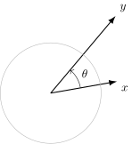
The similarity metric that is most often used in contrastive learning is cosine similarity. Consider the angle between two vectors,
as shown in Figure 120. Then the cosine similarity measures the cosine of this angle,
which captures how well two vectors are aligned on a scale of -1 to 1.
Cosine similarity is related to Euclidean distance in the following sense. If the vectors \(x\) and \(y\) are normalized, i.e., \(\|x\| = \|y\| = 1\), then we can write the squared Euclidean distance as
![The pairwise constrastive loss [38] for similar examples (left) and dissimilar examples (right) for different margins . As can be seen, the loss penalizes simil](assets/diagrams/8ebad48e470aff66.svg)
9.2.1 Loss Functions
Perhaps the most simple objective for learning the parameters \(\theta\) of an embedding function \(f\) is the pairwise contrastive loss proposed by Hadsell et al. [38]. Here we take two samples \(x_i\) and \(x_j\) and define the loss
where \(z_i = f(x_i, \theta)\) and \(z_j = f(x_j; \theta)\) are the embeddings, and \(m\) is a margin hyperparameter that controls how close dissimilar examples are allowed to be before they are penalized. Figure 121 plots the loss.
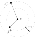
The triplet loss [90, 104] addresses the contrastive learning problem more directly by considering triplets \((x, x^{+}, x^{-})\) containing an anchor training example together with one positive (similar) and one negative (dissimilar) example with respect to the anchor. The loss is then defined as
where the margin hyperparameter \(m\) specifies the minimum gap, i.e., distance, we’d like to obtain between the similar and dissimilar examples. Triplets where this gap is achieved contribute zero to the loss function and hence the gradient during training. The loss is depicted in Figure 122.
This behaviour suggests we need to be careful in choosing our triplets \((x, x^{+}, x^{-})\). Easy triplets will have the negative example far away and hence zero loss. This is computationally wasteful. On the flip side, hard triplets will have the negative example closer to the anchor than the positive example, thus incurring a large penalty and maybe having undue influence on the learning objective. Techniques to mine good examples is critical for the success of learning with a triplet loss, especially when batch sizes are limited and datasets large. Furthermore, the triplet loss requires processing three examples in order to compute one term in the loss function.
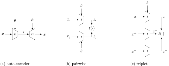
Diagrams comparing the network architectures for representation learning via auto-encoders, pairwise losses, and triplet losses are shown in Figure 123. In the case of the auto-encoder the encoder model \(E\) and decoder model \(D\) have different architectures (yet compatible) each with their own learnable parameters. The branches in the pairwise and triplet loss networks share model architectures and parameters. For the triplet loss, the gradient is only propagated back through the anchor (top) branch.
The InfoSNE loss [77] overcomes the data inefficiencies associated with the triplet loss by selecting only pairs of similar examples and assuming everything else in the batch is dissimilar (i.e., negative). The loss for a pair of similar examples \(i\) and \(j\) is then,
It is instructive to compare this loss to the multi-class logistic and cross-entropy losses from Lecture 2. As with those losses, the InfoNCE loss usually includes a temperature parameter \(\tau\). As the temperature \(\tau\) reduces to zero, probabilities become sharp and hard negatives dominate the loss. This can result in large gradients which destabilizes training. As such, the temperature parameter is annealed during training, starting from a high value and reducing slowly over training epochs.
9.2.2 Obtaining Similar Pairs
We now turn our attention to the problem of obtaining similar pairs for training. In some cases these can come from known labels (e.g., MNIST digits) or inherent property of the data itself (e.g., two nearby frames in a video). However, this is limited to particular data or the need to have human provided labels, which does not scale. A better approach, introduced as SimCLR by Chen and He [15] is to start with a single sample from the dataset and apply random augmentations to that sample to obtain a similar pair. This is depicted in Figure 124. The augmentations—which for images include random rotations, crops, skews and masking—can be performed on-the-fly reducing the need to pre-compute and store the pairs, and allowing for variability in the pairs even when the same sample is seen in the next epoch. For each element in a batch of size \(B\) we generate one positive pair and \(2(B-1)\) negative examples (with respect to that element).
![Network architecture for SimCLR [15]. Here a single sample from the dataset passes through two different data augmentation operations to obtain a pair of simila](assets/diagrams/b5481e530c98cbde.svg)
9.2.3 Caching Old Examples
Naive contrastive learning breaks down at scale due to small batch sizes relative to the number of negative examples needed for good results. Even SimCLR [15] requires very large batch sizes with many thousands of examples for effective learning. However, large batch sizes are expensive in terms of memory and compute—they require distributed training over multiple GPUs, which introduces communication overhead and infrastructure scaling complexities.
One idea is to simply store embeddings from previous batches in a memory bank. This gives lots of negatives without the need for a large batch. Unfortunately simply storing embeddings from previous batches fails because the old embeddings were calculated from old parameters, and hence are no longer reflective of the embeddings that would be obtained from the current model. This is known as representation drift.
MoCo [43] solves this problem by introducing two separate encoders: one for positive examples in the current batch (queries) and one for all other examples in the batch (keys). Since the encoders have the same architecture we can refer to them by their parameters \(\theta\) and \(\phi\). The second encoder, \(\phi\), is updated slowly using an exponential moving average (EMA) filter,
and where \(\theta\) is update using gradient descent as usual. The parameter \(\beta\) is set to a very high value, typically 0.999. This setup keeps the (old) embeddings stored in memory consistent with the newly computed embeddings.
The memory is implemented as a fixed size queue, \(\cQ\). Once the queue fills up, old embeddings are removed to make way for new embeddings. This too mitigates against embeddings getting too stale. The MoCo loss is then an adaptation of the InfoNCE loss where each example in the batch is contrasted against both other examples in the batch and examples stored in the queue,
9.2.4 Avoiding Collapse
All self-supervised learning algorithms run the risk of finding trivial solutions. For example, in representation learning this could be all input examples collapsing to the same embedding (\(\forall x \in \cX,\, x \mapsto z_0\)). Clearly this is undesirable, and many techniques have been developed in contrastive learning to void collapse. We have already seen some of these in the design of the loss functions. Others include:
- feature normalisation
- negative sampling1
- student-teachers branches with exponential moving average (EMA) parameter updates
- strong data augmentation that is task aware
- projection head between the representation and loss
Some advanced techniques promote certain structure in the latent space, e.g., orthogonality, to stop collapse (e.g., Li et al. [64]). Other methods force the model to be able to reconstruct the input from the embedding (i.e., auto-encode) by adding a decoder head and reconstruction loss. This is an old technique but still very effective.