Chapter 3
Back-propagation and Learning
This lecture covers the technology at the heart of deep learning: back-propagation. We begin with a brief review of supervised machine learning and optimization by gradient descent. Then by considering deep learning models as computation graphs, or equivalently function compositions, we show how gradients can be automatically computed. We cover some practical considerations and conclude with an example of putting it all together to learn a simple multi-class classifier.
Recall that in supervised learning we are given a parametrized model \(y = f(x; \theta)\) and a set of training examples \(\cD = \{(x^{(i)}, y^{(i)})\}_{i=1}^{N}\). Our goal is to find the parameters \(\theta\) so that \(f(x^{(i)}; \theta)\) is a good predictor of \(y^{(i)}\) for all \(i=1, \ldots, N\). We do this by defining a regularized loss function \(L\) that measures how well the model fits the training data. The loss function usually decomposed over the training data plus a prior on the parameters,
We then optimize the loss function with respect to the parameters to find the best model
The simplest algorithm for doing this is gradient descent, which iteratively updates \(\theta\) as
where \(\eta\) is a step size, either fixed or chosen via some step size schedule.
The most basic model we can think of in deep learning is the multi-layer perceptron (MLP), which is a composition of affine transformations with elementwise non-linear transforms. Concretely, let \(x \in \reals^{p_0}\) be the input data, \(z_j \in \reals^{p_j}\) be the hidden layer features, and \(y \in \reals^{p_n}\) be the output. Each layer computes its output as
where \(A_j \in \reals^{p_{j} \times p_{j-1}}\) and \(b_j \in \reals^{p_j}\) are parameters, and \(\sigma_j\) is a non-linear activation function. To simplify this expression so that it applies to all layers in the network, we have defined \(x \triangleq z_0\) and \(y \triangleq z_n\). Hence, the multi-layer perceptron defines the composition
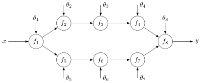
The idea of composing affine functions and non-linear activations in multi-layer perceptrons can be generalised in the sense that the function \(f(\cdot; \theta)\) can be an arbitrarily composition of simple differentiable parametrized sub-functions, and where the parameters of these functions are optimised end-to-end. The composed function can be represented by a computation graph as illustrated in Figure 20, where the sub-functions are depicted as nodes in the graph. This type of representation is very popular for describing deep learning architectures where nodes can denote anything from a very simple arithmetic operation to very complicated algorithmic procedures and data transformations.
To compute the output of the function, we sort the nodes in topological order and evaluate each sub-function in turn,
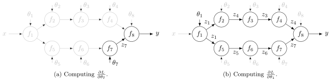
To compute the derivative of a loss function at the output of the graph, with respect to any parameter or input of the graph, we simply apply the chain rule of differentiation by following the arrows backwards through the graph. This is known as back propagation. Two examples are shown in Figure 21 for computing the derivative of the loss \(L\) with respect to parameter \(\theta_7\) and parameter \(\theta_1\), respectively. Here writing out the chain rule we have
where, for the latter derivative \(\frac{\partial L}{\partial \theta_1}\), the first term in the summation is from the top branch and second term in the summation is from the bottom branch of the graph.