Chapter 5
Object Detection and Image Segmentation
This lecture moves from image classification to more sophisticated image labeling tasks—object detection and segmentation. We start by discussing the detection task and how it is evaluated. We then present some simple approaches for building an object detector from an image classification model. These approaches are progressively enhanced to arrive at state-of-the-art object detection methods. Next we introduce image segmentation going from unsupervised over-segmentation to dense semantic and instance pixel labeling. The latter requires fully convolutional networks and upsampling of feature maps through transposed convolutions. We end with a presentation of popular segmentation architectures and models.
The task of image classification studied in the previous lecture works great for images of single objects (or tagging scenes of a particular type like city or rural or forest). We could also imagine a task where we cropped the image around the single object within it, called localization, to make the subject of classification more precisely framed. But most scenes contain more than one object. Object detection is the task of finding multiple objects in an image by placing a bounding box around each object found and assigning a category label to that bounding box. An even more detailed detection and localization task, called instance segmentation, where we outline objects precisely, will be discussed in the second part of the lecture. Figure 49 illustrates the difference between these tasks.
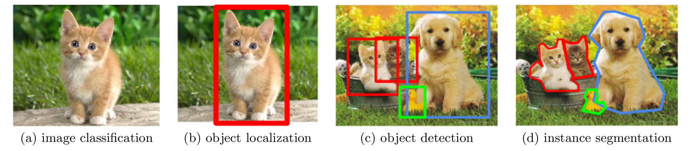
More formally, we can define image classification as the task that takes as input a \((3, H, W)\)-tensor representing a colour image and produces a class label from a set of \(K\) possible classes. The task is evaluated based on an accuracy metric, i.e., how many images were correctly classified from the hold-out test set. The localization task also takes an image as input but produces box coordinates \((x, y, w, h)\) denoting the top-left coordinate of the object \((x, y) \in [0, W-1] \times [0, H-1]\), its width \(w \in [1, W - x]\) and its height \(h \in [1, H-y]\).1 To avoid having to deal with images of different sizes, the box coordinates are usually normalized to between zero and one by dividing box coordinates by image width, \(W\), or height, \(H\), as appropriate.
Since localization is regressing to a 4-dimensional vector (denoting the bounding box coordinates) we cannot simply compare to some exact ground-truth annotation, where a single pixel difference would result in an incorrect prediction. Instead we use a more forgiving intersection-over-union metric that will be discussed shortly. The task of object detection, then, can be summarized as performing both classification and localization, and is therefore scored based on both accuracy (correct class) and localization (correct bounding box) metrics. Moreover, instead of outputting a single category and bounding box, object detection must return a list of category-bounding box pairs, one for each object in the image. An illustration of the difference between the three tasks is shown in Figure 50.

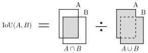
Intersection-over-union (IoU), also called Jaccard index, measures the similarity of two sets. By thinking of bounding boxes as sets of pixels or areas in two-dimensional space, we can use IoU in object detection to determine whether two bounding boxes are close. Given two sets \(A\) and \(B\), we define the intersection-over-union of the sets as,
Note that this is symmetric in \(A\) and \(B\), and is one if and only if \(A\) and \(B\) coincide exactly. IoU is zero if the two sets are disjoint. A graphical depiction of intersection-over-union for two-dimensional bounding boxes is shown in Figure 51 and can be computed in terms of bounding box coordinates as,
where
are the width and height of the intersection between boxes \(A\) and \(B\), respectively.
For a detection to be considered positive it must both predict the correct class label, and have IoU greater than a given threshold, denoted \(\text{IoU}_{t}\), when compared to some ground-truth annotation. Typical thresholds for object detection are 0.3, 0.5 and 0.7 (denoted \(\text{IoU}_{0.3}\), \(\text{IoU}_{0.5}\) and \(\text{IoU}_{0.7}\)), where 0.3 is considered quite loose and 0.7 considered quite tight. To prevent multiple detections of the same object we usually only count the highest probability detection matching with a ground-truth bounding box as correct and all other associated detections as incorrect (even if they have the correct label and IoU above the designated threshold).
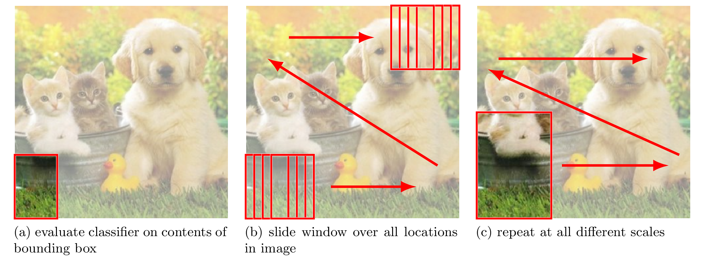
We know from the previous lecture how to design an image classifier, which we can adopt to obtain a class label for the contents of a given bounding box. But where do the bounding boxes come from? One older strategy is known as the sliding window approach. Let us assume that we have an already-trained image classifier. In the sliding window approach, we start by picking some nominal bounding box size and place that bounding box at the corner of the image. We then run our image classifier on the cropped contents of the bounding box (see Figure 52). The classifier is augmented with a background category, which allows the model to decide that there is no object (or too many objects) within in the window. This amounts to \((K+1)\)-way classification for a \(K\)-class object detector.
We then slide the bounding box to the next location in the image and repeat until we have evaluated the classifier at every bounding box location (similar to sliding the filter during 2D convolutions). But this only detects objects at a single scale—the scale defined by the nominal bounding box size. So we increase the bounding box dimensions and repeat sliding the newly sized bounding box over the image and running the classifier on the contents at each location. We keep going until we are satisfied that we have evaluated bounding boxes at all scales of interest.
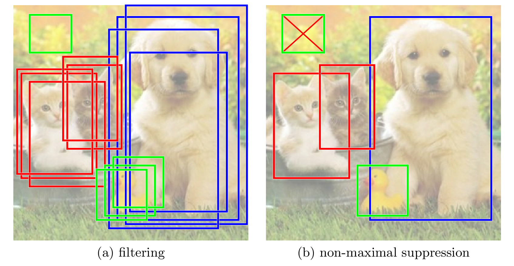
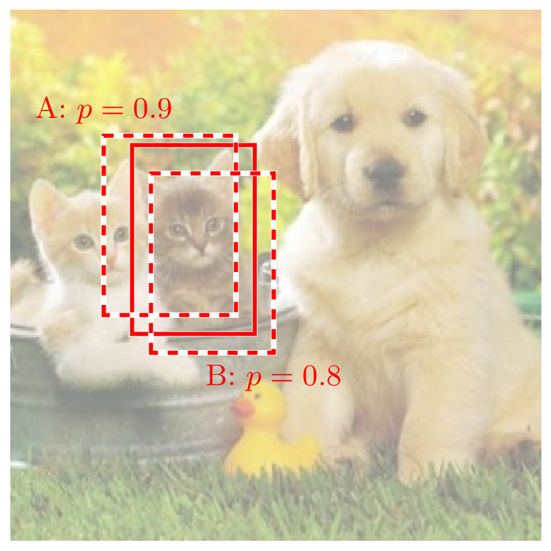
At the end of the sliding window process we are left with a set of bounding boxes of different scales that cover the entire image. Associated with each bounding box is a probability distribution over object classes (and background). The class with highest probability is considered to be the class label for the bounding box. Many boxes overlapping the same object will have high probability (for the same class label) and these need to be handled in some way. The simplest approach is to first filter out low probability bounding boxes and then apply non-maximal suppression (NMS) to get rid of multiple overlapping detections of the same object. See Figure 53. Here bounding boxes are sorted from highest probability to lowest probability. If a bounding box overlaps significantly with a bounding box of higher probability (i.e., preceding it in the list) and having the same label, then the box is removed from the list. This acts to remove overlapping detections of the same object, but in cases of very crowded scenes may also suppress correct detections of nearby objects.
Non-maximal suppression does not get rid of false-positives. Missed detections also cannot be recovered from the filtering and non-maximal suppression algorithm. Mean average precision (mAP) based on some IoU threshold with ground-truth annotations is calculated on the list of remaining bounding boxes to determined the performance of the detector. Repeated detections of the same object are counted as false-positives, meaning that the highest probability detection (that meets the IoU requirement) is determined as correct and the rest as incorrect. See Figure 54. This prevents a detector from gaming the metric by labeling every bounding box as a detection.
While the sliding-window approach is simple, it is very costly due to the large number of times we need to evaluate the image classifier, i.e., once per bounding box. It is a fairly straightforward calculation to count the number of unique bounding boxes of any possible size and placed at any possible location within an \(H \times W\) image. Specifically, the top-left of the box can be anywhere from \(x = 0\) to \(W - 1\) and \(y = 0\) to \(H - 1\). And the width and height of the box can be anywhere from \(w = 1\) to \(W - x\) and \(h = 1\) to \(H - y\). Therefore we have
So, as an example, for a \(1280 \times 720\) image there are \(212 \times 10^9\) unique boxes! Clearly we would like to do better.
The selective search algorithm proposed by Uijlings et al. [99] finds a small set of candidate boxes that are likely to contain objects. The algorithm performs a bottom up over-segmentation and then uses agglomerative clustering to merge similar segments. We won’t go into the details, but the result is 2,000 class-agnostic bounding box proposals per image independent of the image size. This is far fewer than enumerating all possible bounding boxes. However, because the bounding box proposals were found in a class-agnostic way using low-level features they may not align the best for each detected object. We can fix this with a trained bounding box alignment model.
To recap, when performing object detection on an image we take bounding boxes within the image, crop out the region enclosed by the bounding box, resize it, and feed the resized cropped image into a convolutional neural network classifier as if we were performing image classification. At the same time we can perform regression on the bounding box coordinates to improve (i.e., tighten) its localization of the object. Figure 55 shows a canonical architecture to achieve both image classification and bounding box regression. A shared convolutional neural network backbone computes a feature representation of the cropped image. This representation is then fed into two separate branches. The first branch completes the standard image classification pipeline by passing the features through a multi-layer perceptron followed by a softmax classifier. The second branch passes the features through a different multi-layer perceptron that predicts the refined (4-dimensional) bounding box coordinates.

The model is trained end-to-end through the multi-layer perceptrons and shared backbone using a combination of two loss functions. To train the classifier branch we use a cross-entropy (CE) loss on true label, \(y^{(i)}\), whereas to train the bounding box regressor we use a mean-square-error (MSE) loss on true bounding box, \(b^{(i)}\). Here the bounding boxes are adjusted to be relative to the cropped region (which is what the network sees). The second loss is only applied to non-background boxes (determined by IoU with ground-truth). The total training loss over a batch of crops \(\cD = \{(x^{(i)}, y^{(i)}, b^{(i)})\}_{i=1}^{N}\) is then a weighted combination of the CE and MSE losses,
where \(p\) represents the probability distribution estimated by the classifier branch, and \(\theta\) represent the combined parameters of the model, including the parameters of the two multi-layer perceptrons and the backbone convolutional neural network. Here \(\lambda\) is a hyperparameter that controls the trade-off between lower cross-entropy loss for classification and lower mean-square-error loss for better localization, though the two need not be in competition in that tuning the backbone network parameters to reduce one may also help to reduce the other. Note that the parameters of the multi-layer perceptrons in the classifier and bounding box branches are only affected by the losses applied to their branch, cross-entropy and mean-square-error, respectively. The backbone convolutional neural network parameters are affected by both losses.
Training data for the detector comes from manually annotated ground-truth, where a human has gone through and drawn a bounding box around every object in the set of training images and provided a label for each box.2 Crops of these bounding boxes together with crops of proposed bounding boxes obtained from selective search. Any proposed bounding box with sufficiently high IoU with a ground-truth bounding box takes that ground-truth label. Multiple bounding boxes for the same object (i.e., duplicate detections) are allowed during training as these form a type of data augmentation, making the learned model more robust.
- 1. Note the zero-based indexing here. Note also that bounding boxes are sometimes represented by the top-left and bottom-right coordinates, i.e., \((x_1, y_1, x_2, y_2)\) instead of top-left, width and height, \((x, y, w, h)\).
- 2. Sometimes very small objects and highly occluded objects are ignored.