Section 1.2
Machine Learning from 10,000ft

At its core machine learning is about finding a function \(f\) that maps from an input space \(\cX\) to an output space \(\cY\) (see Figure 3). Since we can’t practically search over all possible mappings we define a function class parametrized by \(\theta\) and train a model on a dataset of samples from \(\cX\) and \(\cY\), denoted \(\cD = \left\{\left(x^{(i)}, y^{(i)}\right)\right\}\!{}_{i=1}^{N}\). For example, the function class may be restricted to only linear functions or only polynomials or neural networks of a given architecture. The goal is for the model perform well over the entire space—it is no good to just memorize the training samples. This is, of course, very difficult since much of the space is unseen (i.e., not covered by samples in \(\cD\)). The mapping \(f\) is learned by minimizing (over the parameters \(\theta\) of the model) a loss function \(L\), that in some sense measures the inaccuracy of the model. Typically, the loss function decomposes over sampled input-output pairs,
This is called empirical risk minimization [102].1 Here the loss function \(L\) tells us what to do, and the parametrized function \(f(\cdot; \theta)\) tells us how to do it.2 The objective (composed of the loss \(L\) and the mapping function \(f\)) is, in general, nonconvex in the parameters \(\theta\). As such, we can only hope to find a local minima of the learning problem, which we do using gradient descent or one of its variants.3
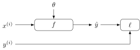
It is common to represent the machine learning model diagrammatically as,4

We can also incorporate the loss function in the diagram when we want to stress how the model is trained,
To summarise, empirical risk minimization (ERM) [102] is a principled framework for choosing model parameters in machine learning. The theory of empirical risk minimization states that we should choose the parameters of the model \(\theta\) that minimize \(L\) over all possible parameters (i.e., the “hypothesis” class). To prevent overfitting on the training dataset or to incorporate prior information into the model we often include a regularization term on \(\theta\),
where \(\lambda\) is a hyperparameter that controls the regularization strength. This is known as regularized empirical risk minimization. The most common regularization function is the squared-norm of the parameters, \(R(\theta) = \frac{1}{2} \|\theta\|_2^2\), which has a nice theoretical interpretation and also results in a simple modification to gradient descent based update rules.
A very common pattern in deep learning is the encoder-decoder paradigm. Here one model, the encoder, maps from the input space \(\cX\) to some latent space \(\cZ\). A second model then maps from the latent space to the output space \(\cY\), as shown in Figure 4. The encoder and decoder models each have their own parameters and can be trained together or separately. Usually the latent space is smaller than the input or output spaces, and hence acts to compress the representation of the data. As a graphical illustration of this, we often draw encoder functions (\(E\)) and decoder functions (\(D\)) as follows,
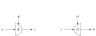
Parameters are often omitted from these diagrams for brevity. Owing to the shape when the diagrams are combined, encoder-decoder models are sometimes called hourglass models.
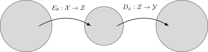
Encoder-decoder models can be divided into auto-encoders, where the input and output spaces are the same and cross-encoders, where the input and output spaces are different. One use of an auto-encoder is to learn a low-dimensional (and sometimes sparse) representation of the data. We do not need explicit supervision for this task since the aim is to reconstruct the input \(x\) from its encoded version \(z = E(x; \theta)\), i.e., we want \(y = D(E(x; \theta); \phi)\) to be close to \(x\). The latent variable \(z\) is called a bottleneck between \(x\) and \(y\).
Cross-encoders have numerous applications. Indeed, many of the recent advances in deep learning and generative AI can be considered as a cross-encoder. With convolutional neural network (CNN) encoders and decoders we can implement semantic segmentation and style transfer algorithms; with recurrent neural network (RNN) encoders and decoders we can implement language translation models; and with a mixed CNN encoder and RNN decoder we can implement image captioning. Multiple different encoders can also be used to learn joint embedding spaces for images and language (e.g., CLIP [83] and BLIP [65]), allowing us to map from one semantic space to another.
1.2.1 Ingredients of a Machine Learning System
There are several ingredients that make up a machine learning system. They should be considered carefully whenever designing, debugging or deploying a system for a specific task. Perhaps the most obvious ingredient is the data, which includes the input signals (i.e., set of images) and the target labels for supervised tasks. The data is used for training as well as evaluating the system, and we need to be sure there is sufficient quantity and quality for both of these roles. How these are represented, that is what datastructures are used for storing and processing, plays an important part of the system design. For example, labels can be represented as text strings, integers (each indexing a list of categories), or one-hot vectors; videos can be stored in a compressed encoded format or as a sequence of extracted frames.
Next, the model architectures (also known as networks) and training objectives (i.e., losses and priors), which we touched on above, are central to the workings of the system. Equally important is the learning algorithm used to tune the model’s parameters using the training data and guided by the training objective. A crucial element of the learning algorithm for deep learning systems is how the parameters are initialised as this can have a big affect on the resulting performance and convergence rate of the algorithm.
Last, is the evaluation metrics. These map our judgment of how a system should perform into quantifiable scores. Using a single measure of performance can often be misleading. For example, reporting detection rates for a positive class (e.g., detecting cancer) and ignoring false positives can be misled by a system that always returns positive. It is important to think critically of the evaluation metrics, what they mean and where they may fail.
Each one of these ingredients—data, representations, architectures, objectives, and metrics—encode (inductive) biases that affect system behaviour and provide levers to change behaviour. We will study each of them in this course in the context of different applications of deep learning.
- 1. The function \(L\) is often scaled by \(1/N\). Technically it is then the expected loss called risk with the function \(\ell\) being the loss. However, most researchers will use the terms interchangeably, or simply refer to any function being minimized in deep learning a loss function.
- 2. Often you’ll see notation \(f_\theta\), indicating that \(\theta\) indexes \(f\) from some function class \(\cF\). However, in these notes we prefer \(f(\cdot; \theta)\) to make it clear that the function takes parameters as an argument and avoid confusion when discussing function compositions in later lectures.
- 3. In practical applications suboptimal solutions are often desirable since finding the globally optimal solution can result in poor generalization of the model to unseen test samples. Techniques such as regularization, data-augmentation, and model selection on a hold-out validation set all help in this regard, and will be discussed in later lectures.
- 4. In the sequel we will sometimes use symbol \(y\) to denote the target output (i.e., groundtruth) and sometimes the estimated output of the network (i.e., as a shorthand for \(f(x; \theta)\)). At other times we will use \(\hat{y}\) for the estimated output. The meaning should be clear from the context.