Section 1.3
Data Representation and Linear Algebra Basics

Deep learning builds heavily on linear algebra (and a bit of differential calculus) for much of its numerical processing. Linear algebra is an incredibly rich area of mathematics and we will only review a few key topics here. We recommend the following online resources for students interested in delving more deeply into the field:

Gilbert Strang’s MIT lectures, https://www.youtube.com/playlist?list=PL49CF3715CB9EF31D
3Blue1Brown animated math videos, https://www.3blue1brown.com/topics/linear-algebra

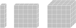
Figure 5: The basic datastructures in deep learning are vectors, matrices and tensors.

The first thing we need to consider is how data is represented and stored. For the purposes of this course (mostly), a (column) vector is a one-dimensional array of numbers, a matrix is a two-dimensional array of numbers, and a tensor is an arbitrary-dimensional array of numbers (see Figure 5). The number of dimensions is called the order of the tensor, so an first-order tensor is just a vector.

The term dimension can also be used to specify the number of entries a vector, e.g., a 3-dimensional vector, but the meaning should be clear from the context. In deep learning we tend to describe vectors, matrices and tensors by their size or shape, e.g., a matrix with two rows and three columns, that is, a 2-by-3 matrix, has shape (2, 3). A matrix with the same number of rows as columns is said to be square.

Figure 6: A colour image is represented using a third-order tensor composed of red, green and blue channels. (Mandrill image from USC Image Database, https://sipi.usc.edu/database/)

An image is an array of red, green and blue (RGB) colour pixels. As such it can be represented by a third-order tensor with integer values in the range 0–255 or floating-point values in the range 0.0–1.0 (see Figure 6). The order in which data is stored is not consistent across software frameworks: In OpenCV and numpy images have shape $(H, W, 3)$, whereas in PyTorch they have shape $(3, H, W)$, where $H$ and $W$ and the height and width of the image, respectively.

We will often refer to a colour image as a 3-channel or 3-plane image. Instead of colour, which can be thought of as a 3-dimensional vector, we can generalize to $C$-dimensional feature vectors for each pixel assembled into a feature map of size $(C, H, W)$, also called a $C$-channel feature map. A video then can be represented using a fourth-order tensor with shape $(3, H, W, T)$, where $T$ denotes the number of frames in the video.

1.3.1 Transpose

Given an $m \times n$ matrix, $A$, we can define its transpose, $A^T$, as the $n \times m$ matrix where the rows and columns of $A$ have been swapped. For example,

\begin{align} A = \begin{bmatrix} A_{11} & A_{12} \\ A_{21} & A_{22} \end{bmatrix} = \begin{bmatrix} 8 & 5 \\ 3 & 6 \end{bmatrix} \qquad A^T = \begin{bmatrix} A_{11} & A_{21} \\ A_{12} & A_{22} \end{bmatrix} = \begin{bmatrix} 8 & 3 \\ 5 & 6 \end{bmatrix} \tag{3}\end{align}

It should be clear from this definition that the transpose of a column vector is a row vector and vice versa, e.g.,

\begin{align} a = \begin{bmatrix} 8 \\ 5 \\ 3 \\ 6 \end{bmatrix} \qquad a^T = \begin{bmatrix} 8 & 5 & 3 & 6 \end{bmatrix} \tag{4}\end{align}

A square matrix that is equal to its transpose is called symmetric. The following properties of transpose are true:

$\left(A^T\right)^T = A$
$\left(AB\right)^T = B^T A^T$
$\left(A + B\right)^T = A^T + B^T$

The idea of transpose extends to tensors where we then also need to specify exactly which channels are being swapped.

1.3.2 Special Vectors and Matrices

Some special vectors up often and can be used to simplify notation, e.g., the all-zeros vector $\zeros_n$ and all-ones vector $\ones_n$. The canonical vector $e_i$ is a vector with all zeros except for the $i$-th location, which contains a one. This sometimes also called an indicator vector or one-hot vector and can be used to denote a category or class label in classification problems.

The same ideas extend to matrices, e.g., $\zeros_{m \times n}$, $\ones_{m \times n}$ and $E_{ij}$ for the zero matrix, all-ones matrix, and indicator matrix with a one for the $(i,j)$-th component and zeros elsewhere, respectively. Another special matrix that you should know about is the diagonal matrix which is a square matrix where the off-diagonal entries are all zeros. The diagonal entries may or may not be zero. When the diagonal entries are all ones the matrix is called the identity matrix and denoted by $I_{n \times n}$. The identity matrix serves the role of one in scalar arithmetic—multiplying by the identity matrix copies the multiplicand to the output.

Subscripts denoting the size of the (zero, ones and identity) vectors and matrices are often omitted when it is clear from the context.

1.3.3 Addition and Multiplication

Two matrices of the same size can be added together in a componentwise fashion so that $C = A + B$ means

\begin{align} C_{ij} &= A_{ij} + B_{ij} \quad \forall i = 1, \ldots m \text{ and } j = 1, \ldots n \tag{5}\end{align}

The product of a matrix $A \in \reals^{m \times n}$ and a vector $x \in \reals^{n}$, written $y = Ax$, is an $m$-dimensional vector with elements

\begin{align} y_{i} = \sum_{j=1}^{n} A_{ij} x_{j} \tag{6}\end{align}

for $i = 1, \ldots, m$. The cost of matrix-vector multiplication is $O(mn)$.

The product of two matrices $A \in \reals^{m \times n}$ and $B \in \reals^{n \times p}$ is an $m \times p$ matrix with elements

\begin{align} C_{ij} = \sum_{k = 1}^{n} A_{ik} B_{kj} \tag{7}\end{align}

for $i = 1, \ldots, m$ and $j = 1, \ldots, p$.

Note that the order of the matrices matters and for the product to exist we need the number of columns of $A$ to equal the number of rows of $B$. However, matrix multiplication is associative, $(AB)C = A(BC)$, and distributive, $A(B + C) = AB + BC$. Matrix multiplication is not, in general, commutative, $AB \neq BA$.

The cost of matrix multiplication in $O(mnp)$.

Consider a matrix $A \in \reals^{m \times n}$ and vector $x \in \reals^n$. We can interpret the product $y = Ax \in \reals^m$ in the following ways:

the $i$-th entry of $y$ is the inner product of the $i$-th row of $A$ (denoted by $a_i^T \in \reals^{1 \times n}$ here) and $x$
$\begin{align*} y \quad = \quad \left[ \begin{matrix} \text{--- } a_1^T \text{ ---} \\ \text{--- } a_2^T \text{ ---} \\ \vdots \\ \text{--- } a_m^T \text{ ---} \end{matrix} \right] x \quad = \quad \left[ \begin{matrix} a_1^T x \\ a_2^T x \\ \vdots \\ a_m^T x \end{matrix} \right] \end{align*}$
$y$ is a linear combination of the columns of $A$ (denoted by $a_i \in \reals^{m}$ here for the $i$-th column)
$\begin{align*} y \quad = \quad \left[ \begin{matrix} | & | & & | \\ a_1 & a_2 & \cdots & a_n \\ | & | & & | \end{matrix} \right] x \quad = \quad \sum_{i=1}^n x_i a_i \end{align*}$

1.3.4 Inner Product and Euclidean Norm

The inner product between two vectors (of equal length) is defined by

\begin{align} \left<x, y\right> &= x_1 y_1 + \cdots + x_n y_n \tag{8}\\ &= x^T y \tag{9}\end{align}

Some important properties of inner product are:

$\left<\alpha x, y \right> = \alpha \left<x, y \right>$
$\left<x + y, z \right> = \left<x, z \right> + \left<y, z \right>$
$\left< x, y \right> = \left<y, x \right>$
$\left< x, x \right> \geq 0$
$\left< x, x \right> = 0$ if and only if $x = 0$

The row vector $x^T$ represents a linear function $\reals^n \rightarrow \reals$.

For $x \in \reals^n$, we define the (Euclidean) norm as

\begin{align} \|x\|_2 &= \sqrt{x_1^2 + \cdots + x_n^2} \tag{10}\\ &= \sqrt{x^Tx} \tag{11}\end{align}

The quantity $\|x\|_2$ measures the length of the vector (from the origin).

Some important properties of norm are:

$\| \alpha x \| = |\alpha| \|x\|$
$\| x + y \| \leq \|x\| + \|y\|$ (triangle inequality)
$\|x\| \geq 0$
$\|x\| = 0$ if and only if $x = 0$

Other important (vector) norms are $\|x\|_1 = |x_1| + \cdots + |x_n|$ and $\|x\|_\infty = \max\{x_1, \cdots, x_n\}$.

1.3.5 Batch Processing and Broadcasting

Deep learning frameworks process data in batches, passed as tensors. The first dimension of the tensor is the batch dimension. So, for example, a batch of $n$-dimensional vectors has shape $(B, N)$, and a batch of colour images has shape $(B, 3, H, W)$.

Example. For the operation $y = Ax + b$ we might have

\begin{align} X &= \{x^{(1)}, \ldots, x^{(B)}\} & \text{(input)} \tag{12}\\ Y &= \{Ax^{(1)} + b, \ldots, Ax^{(B)} + b\} & \text{(output)} \tag{13}\end{align}

Many PyTorch functions are batch-aware and support broadcasting where data along singleton dimensions is automatically replicated to match arguments within an operation, e.g., for $(M \times N)$-matrix $A$, $M$-vector $b$, and batch of $N$-vectors $x$,

y = torch.matmul(A.view(1, M, N), x.view(B, N, 1)).view(B, M) + b.view(1, M)
# could also be done with: y = torch.einsum("ij,kj->ki", A, x) + b

computes $y^{(k)} = Ax^{(k)} + b$ on each element $k = 1, \ldots, B$ of the batch.

1.3.6 Tensors in PyTorch

In addition to their shape (size), tensors in PyTorch have several other properties:

dtype to specify numerical precision, e.g., 32-bit float
device, e.g., on CPU or GPU
requires_grad will be discussed later
grad holds gradient for training (will be discussed later)

There are many ways to create a tensor. For example,

A = torch.tensor([[8, 5], [3, 6]])

creates the matrix

\begin{align} A = \begin{bmatrix} 8 & 5 \\ 3 & 6 \end{bmatrix} \tag{14}\end{align}

A Parameter is a type of learnable Tensor used within PyTorch modules that you will encounter later in the course.

It will often prove useful to be able to reshape a tensor when implementing deep learning models. Reshaping is always possible so long as the total number of elements does not change, e.g.,

A = torch.tensor([[8, 5, 1], [3, 6, 2]])
B = A.reshape([3, 2])

creates matrices

\begin{align} A = \begin{bmatrix} 8 & 5 & 1 \\ 3 & 6 & 2 \end{bmatrix} \quad \text{and} \quad B = \begin{bmatrix} 8 & 5 \\ 1 & 3 \\ 6 & 2 \end{bmatrix} \tag{15}\end{align}

Note that this is different to transpose, which would create

\begin{align} A^T = \begin{bmatrix} 8 & 3 \\ 5 & 6 \\ 1 & 2 \end{bmatrix} \tag{16}\end{align}

from PyTorch code

A.transpose(0, 1)

The method view can also be used whenever the memory layout of the underlying data does not need to change, e.g., B = A.view([3, 5]).

A very common reshaping is to flatten the tensor (sometimes called vectorizing), e.g., C = A.flatten() produces

\begin{align} C &= \begin{bmatrix} 8 & 5 & 1 & 3 & 6 & 2 \end{bmatrix} \tag{17}\end{align}

Note that elements are rearranged rowwise (called row-major ordering).

1.3.7 Coordinate Systems

A final comment on indexing and coordinate systems. In mathematics we generally index from 1, whereas in code we generally index from 0. This is a source of endless confusion and bugs. Now you know you wont fall into this trap.

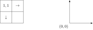
To add further confusion, in linear algebra we index matrices and tensors from top-left to bottom-right, i.e., the top-left element of an $m \times n$ matrix is the $(1, 1)$-th entry and the bottom-right element is the $(m, n)$-th entry. Since we represent images as tensors, this will also be the default indexing for pixels. So the top-left pixel is the first pixel in the image. However, in geometry, coordinate systems increase upwards from the origin. In this coordinate system it is the bottom-left pixel that is the first pixel in the image. Be aware that different tools and different authors may use different coordinate systems. If you view an image and everything is upside down then flip the coordinate system.

Section 1.3Data Representation and Linear Algebra Basics