Section 7.2
Algorithmic Issues

Other issues that we should be aware of are algorithmic issues, including poor experiment design (e.g., choosing a favourable random seed), systematic error from mini-batch sampling or division into train-test split, and leaking information from test set during training. Let’s consider these one at a time.

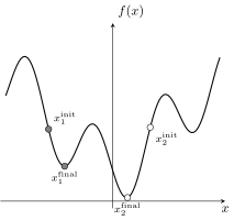
Objective functions in deep learning are, in general, non-convex so we cannot hope to optimize them fully. Indeed, we are often satisfied with a local optimum of our loss functions. And even then, a better value of the loss function on the training set does not always translate to better performance on the test set. Putting the problem of generalization to the side for the moment, consider the task of minimizing the function \(f\) shown in Figure 95. Providing that the function is sufficiently smooth and we take small enough steps, gradient descent will take us from the initial point to the nearest local minimum. As such different initializations will lead to different solutions, and it is not hard to see that a lucky random seed can favour or penalize one model over another. To mitigate against this it is important to always repeat experiments initializing with different random seeds and report statistical results (mean and standard deviation over performance metrics). You should also try to run controlled experiments when comparing different variants of a model (e.g., by changing one thing at a time and running the variants with the same random seeds, which has the added advantage of making your results reproducible).

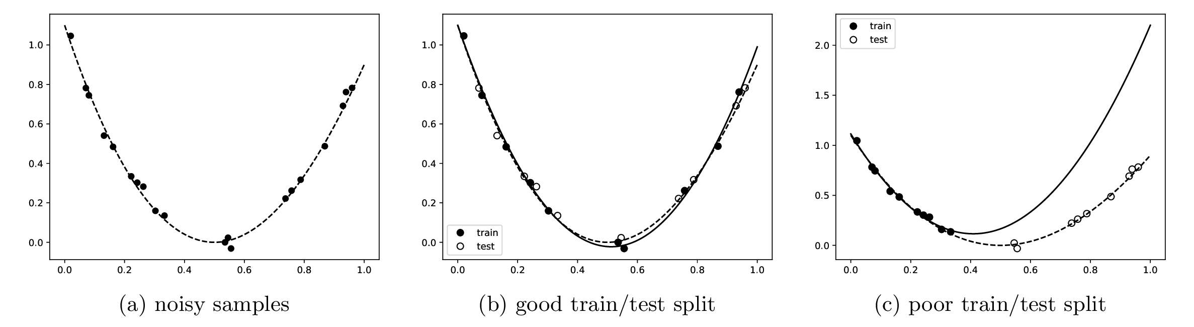
Data sampling strategies can have a big influence on results. A key tenet in machine learning is that the training sample distribution should match test sample distribution (or population distribution). If this is not the case then the learned model will fail to generalize to unseen data. Figure 96 illustrates this idea. Given a set of noisy samples for curve fitting (a), if we split the samples so that they are distributed well over the input domain (b), then the model will generalize well as indicated by its performance on the hold-out test set. However, if we sample in a way that covers only a portion of the input space (c), then the model will perform poorly at test time.

It is important that sampling strategies are designed for the given application. For example, when curve fitting it may be appropriate to alternate every second data point between the training and test sets. But this would be a very poor strategy when sampling frames from a video, for example, since there is very high correlation between consecutive frames and a model trained on such high-dimensional data may end up simply over-fitting to the training data. The high correlation between train and test sets then gives an overly optimistic estimate of generalization performance. A better strategy in this case is to split data at the video level rather than the frame level.¹

A similar thing can happen during stochastic gradient descent if we don’t shuffle data within the training set between epochs. The model, repeatedly seeing data in the same order, will bias performance to data seen at the end of the epoch rather than the start. This is why we always reshuffle data² and apply different data augmentations when training models over multiple epochs.

Another sampling problem occurs when data is not balanced across categories in classification problems. In such situations rare categories may have very different distributions between train and test splits, violating the previously mentioned tenet underlying machine learning. Here a common solution is to use stratified sampling, which is to randomly split data between training and test sets sampling within each class separately rather than the entire dataset globally. The idea is illustrated in Figure 97. Note that there is still imbalance between the classes, but at least the training and testing distributions match. The approach can also be applied when constructing mini-batches during stochastic gradient descent. To deal with class imbalance, reweighting of rare samples in the loss function or sampling with replacement (combined with data augmentation) can also be used.

Test data should never be seen during training or development of the model. This is very difficult to achieve in practice where standard benchmarks use fixed test sets and there is a natural tendency to build on models that work well based on performance reported on the test set. Nevertheless, we can ensure that the training algorithm does not have access to information about the test set. An area where this is often overlooked and hence a common source of information leakage is when pre-processing data. For example, when whitening input data, the mean and standard deviation should be computed using the training data only not the entire dataset. Normalization using these statistics are then applied to examples across the whole dataset.

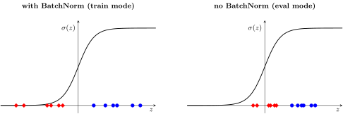
Another common mistake is not putting models into evaluation mode at test time. For example, BatchNorm, should use learned parameters on test data, not parameters estimated from the test batch. This is done using the .eval() method on the model, and instructs the model to keep parameters fixed. For most tasks, the test data is assumed to be independently and identically distributed. Moreover, it should not matter in which order the data is processed, or whether each example is processed individually or in a batch. Figure 98 demonstrates why this may matter if we have not put the model into evaluation mode. The figure depicts a batch of positive and negative examples. With BatchNorm in training mode, the data will be normalized to have zero mean with respect to the batch. This may unfairly favour prediction of samples in the batch. Information from the test set has leaked into the evaluation process. On the right of the figure we see the scenario where we have set BatchNorm to evaluation mode. No information leakage occurs in this case.

7.2.1 Bugs in Machine Learning Algorithms

Bugs in machine learning algorithms can be notoriously difficult to find. This is because machine learning algorithms are inherently trying to optimize for good solutions, so if an algorithm is making progress towards a solution (i.e., minimizing a loss function) then it appears to be working as expected. Consider, for example, trying to minimize the following scalar-valued function

We will use a damped Newton’s method, which is a second-order optimization algorithm with updates

To illustrate the difficulty of debugging, let us introduce a small bug into our implementation of the first- and second-order derivatives. The true derivatives are

but we may accidentally implement our model with the incorrect sign on the second term,

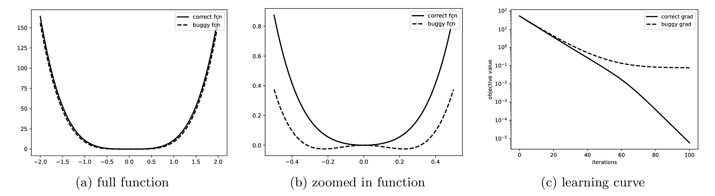
This sort of bug is not uncommon in numerical applications, and in this example would correspond to the function, \(\tilde{f} = 10x^4 - x^2\), which on a macroscopic scale looks very similar to the true function, \(f\), as shown in Figure 99(a). It is only when we zoom in around the minimum that we see a difference (see Figure 99(b)). The manifestation of this bug, is that when we try to optimize using the buggy implementation we fail to converge to the true optimal solution as illustrated when we compare learning curves of the correct implementation against the buggy one in Figure 99(c).

The take home message from this example is to use automatic differentiation wherever possible. More generally, however, produce lots of plots and perform lots of tests. We will discuss some useful diagnostics that will help discovering bugs later in the lecture.

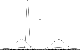
Sometimes you may think you have a bug in the code, but the result of your algorithm is quite reasonable for what your are asking it to do. A very good example is the pathological case of fitting a mixture of Gaussians as illustrated in Figure 100. The aim of fitting a mixture of Gaussians is to represent the empirical distribution defined by a set of samples by the weighted combination of Gaussian probability distributions. This is often used to identify clusters in the data under the assumption that each cluster can be well represented by a single Gaussian. Fitting the mixture solves the following optimization problem for a set of data points \(\{x^{(i)} \in \reals^n\}_{i=1}^{N}\) and \(K\) mixture components,

where \(\pi_k\), \(\mu_k\), and \(\Sigma_k\) are parameters of the model. That is, we find the parameters that maximize the log-likelihood of the data when represented by a mixture of Gaussians.

It turns out that the true optimal solution to this problem is to place a very narrow Gaussian over one of the data points so that it’s likelihood approaches infinity and spread the remaining Gaussian components over the rest of the data. While this maximizes the log-likelihood it is, unfortunately, not the solution that we really want. Most of the time, if we initialize randomly and use gradient descent (or an alternative optimization algorithms known as expectation-maximization [20]), we will converge to a local optimum, which is more desirable.

All this is to say that if your algorithm results weird output it may not be because of a bug. Ask yourself if what you are seeing is reasonable, or just possible, based on what you are asking the machine to do. The simple example above of fitting a mixture of Gaussian is the exact same thing that occurs in a phenomenon known as mode collapse in self-supervised deep learning.