Section 8.1
Tokenization
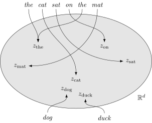
The transformer models was originally designed for natural language processing tasks, and as we saw in the last lecture, the first step in being able to process language data is to encode text into a form amenable for numerical calculations in a deep learning model. The mechanism for converting symbolic data into vectors is called tokenization. One way to think about this is as a mapping from the discrete set \(\{1, 2, \ldots, m\}\) to the space of \(d\)-dimensional vectors, \(\reals^d\). Here each element in the set \(\{1, 2, \ldots, m\}\) indexes a discrete item from the universe of symbols, e.g., a vocabulary of words or \(n\)-grams. An example is shown in Figure 107.
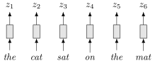
To make this more concrete, let \(E: {\cal V} \to \reals^d\) be an encoder from fixed vocabulary \({\cal V}\) to \(n\)-dimensional vectors. This can be implemented, for example, via a lookup table. Then a sequence of \(T\) words \(\langle w_t \in {\cal V} \mid t = 1, \ldots, T\rangle\) gets encoded as a sequence of tokens \(\langle z_t = E(w_t) \in \reals^d \mid t = 1, \ldots, T\rangle\), as illustrated in Figure 108. In practice, we tokenize sub-words (or \(n\)-grams) rather than full words. Pre-processing is sometimes carried out before converting a piece of text into a sequence of vectors to reduce words to their stems, i.e., part of the word that captures lexical meaning, filter stop words, i.e., common words that carry little meaning, or compress whitespace. However, this has become less important for massive models trained on internet-scale data.
We can also decode from tokens back to words using a decoder model, \(D: \reals^d \to \cV\). Here we need to worry about the fact that some vectors in \(\reals^d\) may not correspond to vectors hit by the encoder \(E\). Mathematically, we say that the encoder function \(E\) is not surjective, meaning that it only maps onto part of \(\reals^d\). There are two standard approaches to get around this difficulty. The first approach is to take the nearest encoded vector to an arbitrary vector \(z \in \reals^d\),
which effectively divides \(\reals^d\) into piecewise constant regions associated with each word \(w \in \cV\). The second approach is to treat the decoder as a stochastic function. Instead of a deterministic decoder function \(D\), we define (or learn) a discrete distribution \(P_D\) over the embedding space and sample a word from this discrete distribution,
For example, if \(z\) and \(E(w)\) are both normalized, then we could define \(P_D\) as
There are several research works that propose how to assign vectors to words, i.e., how to structure the embedding space. In the skip-gram model [71], the high-level idea is to train an encoder model on a large text corpus, \(\cT\), with the desired property that words appearing close to each other in the corpus should have vector representations that are close to each other in embedding space. Consider word \(w_i\) with neighbouring words
for some neighbourhood size \(n\), e.g., \(n = 4\). We want \(w_i\) to be a good predictor of \(w_j \in \cN_i\), i.e., we want to maximize the log-likelihood of the conditional probability of adjacent words to a given word for every word in the corpus,
Given a training text corpus \(\cT\), this is a self-supervised objective. The distribution \(P\) can be modelled as the softmax over embedding similarity, i.e.,
where \(z_i\) and \(z_j\) are the vector representations of \(w_i\) and \(w_j\), respectively, and are the free parameters to be optimized.
Many others approaches and variants of this idea have been proposed, such as GloVe [81] and BERT [22]. For the purposes of these lectures, we will assume that a pre-trained embedding model is supplied, and that the embedding space also contains special tokens such as the start-of-sequence and end-of-sequence tokens discussed in the last lecture.
8.1.1 Positional Encoding
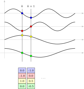
In addition to encoding a word (or \(n\)-gram) as a vector, transformers also encode the location that each word appears in the sequence. This is done with a clever technique known as positional encoding. Here, the \(k\)-th position in a sequence is encoded as a \(d\)-dimensional vector \(\psi_k\) with \((2i)\)-th and \((2i+1)\)-th elements1 determined as
for \(i = 0, \ldots, \frac{d}{2} - 1\). The elements in the positional encoding vector represent a geometric progression of wavelengths from \(2 \pi\) to \(2 \pi n\) as illustrated in Figure 109 (Vaswani et al. [103] set \(n = 10^4\)).
The position encoding vectors are added to the word embedding vectors for each token to give
as the vector representation of the token at the \(k\)-th position.
The transformer architecture itself has no notion of order.2 As such, without positional encoding (or masking, which we will see later) the transformer is technically a set processing model rather than a sequence processing model. Positional encoding allows the model to reason about the order of tokens in the set, thus defining a sequence.
A new type of positional encoding called rotational positional embeddings (RoPE) [95] has become popular in recent years. This replaces the standard additive positional encoding with a multiplicative rotation that preserves relative distance between tokens when performing scaled-dot product attention, i.e., shifting two tokens along a sequence shouldn’t change their relative distance. Details can be found in Su et al. [95] for the interested student.