Section 8.3
Scaled Dot-product Attention

At the heart of the transformer model is a mechanism known as scaled dot-product attention [103]. It replaces the recurrence or convolutions we saw in previous sequence-to-sequence models. The basic idea is shown in Figure 111(left) and can be thought of as a soft content-addressable memory. Let \(q_i \in Q\) be some query vector. Then compute the similarity between \(q_i\) and every key \(k_j \in K\) by computing dot-products, \(q_i^T k_j\). Return a weighted combination of values \(v_k \in V\), where weights are determined by softmax applied to the similarity scores with appropriate temperature scaling.

Multiple queries can be processed simultaneously. If we arrange queries, keys and values as rows in a matrix,

then we can write scaled dot-product attention as

Here the softmax operation is applied row-wise with temperature \(\tau = \sqrt{d}\), where \(d\) is the dimensionality of the query and key vectors. This helps to keep the softmax values in a reasonable range.¹ Note that keys and values are in a one-to-one correspondence with each other. The number of output vectors (or tokens) is equal to the number of queries, and the number of input vectors (or tokens) is the same as the number of keys and values. Typically in a transformer model we set the number of inputs to be the same as the number of outputs (\(m = n\)) and the dimensionality of the output vectors to be the same as the dimensionality of the input vectors (\(p = d\)). As we will see shortly, the queries, keys and values come from tokens in a sequence. But before that let us study the attention function in greater detail.

The first operation in the attention function is to compute the similarity between all queries and keys,

Here each row corresponds to matching a single query, \(q_i\), with every possible key, \(k_j\) for \(j = 1, \ldots, n\). Applying softmax row-wise gives

where each row can be thought of a providing a normalized weight vector \(a_i \in \reals^n\). Finally, the attention function constructs each output as a weighted combination of the value vectors, \(\{v_1, \ldots, v_n\}\),

That is, the \(i\)-th output is constructed as

where \(\alpha_j\) is the \(j\)-th component of \(a_i\). The transpose in the equations above come from the fact that we have arrange the inputs and outputs as rows.

8.3.1 Masking

Without masking every token can attend to every other token in the sequence. Masking allows us to control how each token interacts with other tokens so can be used, for example, to enforce causal attention—output tokens can only be affected by input tokens that appear earlier in the sequence.

The masked attention operator is defined as

where \(M \in \{0, 1\}^{m \times n}\) is a 0-1 matrix. This is equivalent to setting masked values in \(QK^T\) to \(-\infty\) and then applying softmax as we did with unmasked attention since \(e^z \to 0\) as \(z \to -\infty\), i.e., the value vectors corresponding to masked entries receive zero attention weight.

To implement causal attention we can provide a lower triangular mask with all non-zero elements equal to one,

Other sparsity patterns are also possible and may be used depending on the application.

8.3.2 Multi-head Attention

If the attention mechanism is so good, then maybe more of them will be better. Multi-head attention performs dot-product attention on multiple smaller dimensional queries, keys and values in parallel. We have,

for \(j = 1, \ldots, h\) where \(h\) is the number of heads. The queries, keys and values for each head are linear transformations of the original queries \(Q\), keys \(K\) and values \(V\). Here \(W^{(Q)}_j\), \(W^{(K)}_j\) and \(W^{(V)}_j\) are the parameters of the linear transform.² Note that in the expression above we post-multiply by the parameter matrices to perform the linear transform since tokens are arranged row-wise.

An illustration of multi-head attention is shown in Figure 111(right). Each head produces an output \(Z_j \in \reals^{m \times p}\) (where \(m\) is the number of inputs). These outputs are linearly combined to produce the final output of the multi-head attention layer as,

where \(W^{(O)} \in \reals^{hp \times d}\) are learnable parameters. Once again we post-multiple. Usually we set the dimensionality of each head to \(p = d/h\).

8.3.3 Self-attention versus Cross-attention

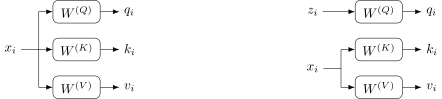
Let us return to the question of where the queries, keys and values come from. We saw at the start of the lecture that we can tokenize a sequence of, say, words, and represent them as vectors in \(n\)-dimensional space. Each of these tokens is associated with a query, key and value, which we obtain via a linear transform. For the \(i\)-th token we have,

or more succinctly,

where as usual for transformers we have stacked tokens (transposed) row-wise to form \(X\).

This is called self-attention because the queries come from the same source of information as the keys and values. An alternative mechanism is cross-attention where the queries are constructed as a linear function of tokens from another branch (i.e., separate input sequence),

where \(\langle x_1, \ldots, x_m\rangle\) and \(\langle z_1, \ldots, z_{m'}\rangle\) are different sequences. An illustration is shown in Figure 112.

8.3.4 Visualising Attention

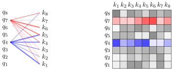
There have been various attempts to understand the workings of transformers by visualising the attention mechanism. Here researchers are usually interested in which input tokens influence which output tokens. Ignoring multi-head attention, recall that an output token is generated by comparing its query with keys for every other token and then using the normalized similarity to form a weighted combination of associated values,

So one way to visualise the influence of tokens on each other is to visualise the attention weights as show in Figure 113. This can also be done by displaying the attention matrix as a heat map, and various other visualisation techniques have also been proposed in the literature.