Section 10.1
Policies, Rewards and Values
Let \(\cS\) be the set of all possible world states and \(\cA\) be the set of actions that an agent may take. The rule that the agent uses to decide on an action is known as a policy. Mathematically, a policy is a function that maps states to actions and is traditionally denoted by the symbol \(\pi\),
A reward function maps each state (or in some models a state-action pair) to a real number,
Since the agent receives a reward, possibly zero, after taking each action, it accumulates these rewards over time. A value function is the total expected reward that an agent will receive by following a policy \(\pi\) after starting in a particular state \(s_0\),
We are now ready to formally define a Markov decision process (MDP) as a tuple \((\cS, \cA, P(s_{t+1} \mid s_t, a_t), \gamma, R)\) where \(P(s_{t+1} \mid s_t, a_t)\) is the transition function that captures the probability of ending up in state \(s_{t+1}\) if the agent takes action \(a_t\) when in state \(s_t\). The parameters \(\gamma\) is called the discount factor and will be discussed later in the lecture.
A simple example of an MDP involves navigating in a grid world by moving to adjacent cells and collecting rewards as shown in Figure 128. The agent does not need to remember its history of previous moves; it decides on an action based solely on its current location in the grid \(s_t\) and a known reward function \(R\). There are two policies shown in Figure 128. The first has the agent move up if if can, otherwise it moves right, otherwise south, and otherwise west. We assume that the agent will always stop at the top-right corner of the grid (which is also where the only positive reward is received). This policy is not optimal. For example, the agent can get stuck in the corridor leading to the dead-end at location \((3,3)\). An optimal policy \(\pi_{*}\) is illustrated in Figure 128(c) where, again, we assume that the agent must stop when it reaches the top-right corner. The policy is optimal in the sense that no matter where the agent starts, the policy will ensure that it maximizes its total reward over the sequence of actions it takes. This sum of rewards is captured by the value function (for a given policy).
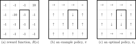
Figure 129 shows how we can calculate the value function for the first (non-optimal) policy and the given reward function.1 Starting in state \((1,1)\), i.e., the bottom-left corner and following the policy the agent moves up the leftmost column and then along the top row accumulating rewards \((-1, -1, -1, -1, -1, -1, 10)\) as it goes. The sum of these rewards is the value assigned to state \((1, 1)\) for this policy. That is, \(V_\pi(1, 1) = 4\). We can repeat this calculation for other starting locations in the grid to obtain their values. Note the \(-\infty\) values that get assigned when the agent gets stuck in the corridor mentioned earlier.
Different policies will have different value functions. For example, an optimal policy \(\pi_*\) will escape the dead-end corridor and thus not incur \(-\infty\) values. Optimal policies also avoid the large negative reward \((-10)\) at location \((2,3)\), instead choosing to go down or left from location \((2,2)\) rather than up. We will show how to find an optimal policy later in the lecture. For now we leave it as an exercise to compute the value function for the optimal policy shown in Figure 128(c).

- 1. In this example the sum of rewards is deterministic since the transition function is deterministic—we know where the agent will be after taking action \(a_t\) in state \(s_t\). If the transition function were probabilistic, i.e., the action could fail and we end up in a different state \(s_{t+1}\), then we would need to compute the sum of expected rewards.