Section 10.3
Finding an Optimal Policy
As we have just seen, the value function is the expected return starting in state \(s\) and following policy \(\pi\) thereafter. We can define another function, known as the quality function or simply \(q\)-function that is the expected return of starting in state \(s\), taking action \(a\), and then following policy \(\pi\) thereafter,
Knowing the \(q\)-function we can easily obtain the value function by summing over actions
Both \(V_\pi\) and \(Q_\pi\) can be estimated from experience, and this allows us to train models and find optimal policies using reinforcement learning. To do so, we sample trajectories,
over which the expectations for \(V_\pi\) and \(Q_\pi\) are taken. When a policy \(\pi_\theta\) is used to generate a trajectory we call it a roll-out or episode. So the value function, in terms of expectations over trajectories, is
where \(P_\theta(\tau) = P(s_1) \prod_{t=1}^{T} \pi_\theta(a_t \mid s_t) P(s_{t+1} \mid s_t, a_t)\).
An optimal policy \(\pi_*\) is one that leads to better rewards than any other policy \(\pi\). In terms of its value function and Q-function, we can write
Given \(Q_*\) we can obtain the corresponding optimal policy as
The optimal value is the current reward plus the optimal value starting at the next state. This is known as the Bellman principle, which can be expressed by the following equation for MDPs,
10.3.1 Value Iteration
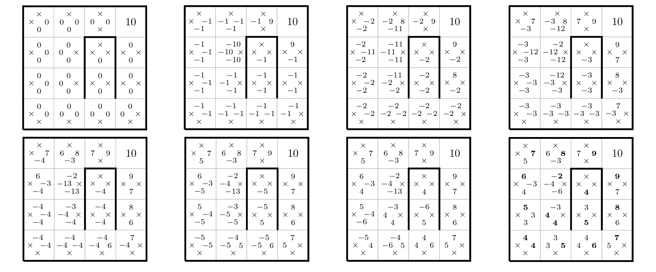
Value iteration is a dynamic programming method used to find the optimal value function \(V_*\) or optimal q-function \(Q_*\). It works by repeatedly applying the Bellman equations to iteratively update estimates of \(V\) or \(Q\). The algorithm can be run synchronously, where values for all states (and actions) are updated at once, or asynchronously, where values are updated one at a time. In both cases the algorithm is guaranteed to converge to the optimal values. Below we given the synchronous version for finding \(Q_*\).1 As \(i \to \infty\), \(Q_i\) converges to \(Q_*\).
Value iteration is conceptually important and valuable for small problems where we have complete knowledge of the MDP, i.e., the transition function. For problems with large state and actions spaces it becomes intractable.
10.3.2 Temporal-difference Learning
Temporal-difference (TD) learning [97] is a method for estimating the value function that learns directly from experience. It therefore overcomes the scale problem and need for complete knowledge that value iteration requires. In most problems we do not fully understand how the environment behaves and so need to perform actions to figure it out. TD learning uses samples state-action-state triplets \((s, a, s')\) to update the value function or \(Q\)-function as
where \(\alpha\) is a learning rate parameter. It can be thought of as a stochastic approximation to the Bellman equation.
10.3.3 Exploration versus Exploitation
When learning the value function (and hence optimal policy) an agent must decide between taking the action that seems to be the best right now or trying something new that might lead to better rewards later. Taking the former actions is known as exploitation whereas taking the latter actions is known as exploration. Exploitation, characterized by the following mathematical expression,
maximizes the agent’s immediate reward (under the current model \(Q\)) but may miss better actions that it has not yet tried. Exploration on the other hand chooses an action by randomly sampling from some action distribution,
and can thus lets the agent gather information about the world. However, it may reduce short-term reward and most actions may not lead to fruitful parts of the state space.
There exists a mathematically difficult trade-off between exploration and exploitation. If you always exploit then you may get stuck with a sub-optimal policy; if you always explore then you do not capitalize on what you have learned. One common solution is called the \(\epsilon\)-greedy approach. Here the agent chooses to explore with probability \(\epsilon\) and otherwise exploit. This simple approach is surprisingly effective.
- 1. It is synchronous because we use \(Q_{i-1}\) to compute \(Q_i\) for each state and action. If instead we overwrite a single \(Q\) buffer then the algorithm becomes asynchronous.