Section 2.1
Logistic Regression
Roughly speaking, logistic regression turns an affine function of the input into a probability distribution over outputs. Let \(y \in \{0, 1\}\) be a random variable with distribution defined by
where \(a\) and \(b\) are parameters and \(x \in \reals^n\) is the observed feature vector. The maximum likelihood principle states that we should choose parameters \(a\) and \(b\) that maximizes the probability of the observed data under the model,
In practice, we (equivalently) minimize the negative log-likelihood function instead,
which is convex in variables \(a \in \reals^n\) and \(b \in \reals\).
The logistic function is an s-shaped curve (sigmoid) that maps from real numbers to the interval \([0,1]\). It is therefore useful for modeling binary probability distributions. An extension of the logistic function is the so-called softmax function, which we will see later. The definition of the logistic function for scalar variable \(z \in \reals\) is,
Replacing \(z\) with \(a^Tx + b\) allows us to learn a probability distribution conditioned on vector-valued features \(x \in \reals^n\),
as we have done above. A property of the logistic function is that \(\sigma(z) \geq 0.5\) if, and only if, \(z \geq 0\). So a classification rule \(a^Tx + b \geq 0\) corresponds to \(P(y \mid x) \geq 0.5\), i.e., predict positive on an input \(x\) if the probability is above 50%.
An illustration of the logistic function for scalar \(z = a^Tx + b\) and two-dimensional features \((x_1, x_2)\) is shown in Figure 8. Observe that the function is bound between zero and one. Note also that for the two-dimensional case (and higher-dimensions) when we look along the \(a\) direction we get a one-dimensional logistic curve.

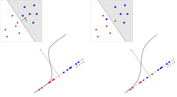
Revisiting our example of binary classification over two-dimensional data, we can now see what a logistic function fitted to the data might look like as illustrated in Figure 9. Notice that in the separable case the logsitic curve is much sharper than in the non-separable case. In fact, in the separable case the function can be made arbitrarily sharp as we continue to train the model. In the non-separable case, the value of the logistic function gives us an estimate of the probability of an example being labeled positive.
Having our classifier too confident around the decision boundary, even in the separable case, is undesirable. Remember we are fitting to a set of training data, and what we really want is for our model to generalise to unseen test data. One way to reduce the confidence of the classifier on positive and negative training examples is through regularization. Here we add a penalty on the magnitude of the model’s parameters, and minimize the resulting combination of loss function and regularizer,
Note that we have not put any regularization on the offset, or bias, parameter \(b\).
This type of regularization is also called weight decay because of it resulting in pushing the parameter values towards zero as evident when considering the gradient of the regularized loss,
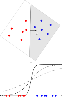
Ignoring the \(\nabla_a \ell\) term for the moment, then taking a step in the negative gradient direction will change parameter \(a\) to \((1 - \eta \lambda) a\), where \(\eta\) is the gradient step size (or learning rate), to be discussed later in the lecture. That is, regularization tends to push \(a\) to zero. From the definition of the logistic function in Equation \(\ref{eqn:logistic_fcn}\) it should be clear that as parameter \(a\) approaches zero, the value of the logistic \(\sigma(a^Tx + b)\) approaches a constant, i.e., \(\frac{1}{1 + e^{-b}}\). Hence, regularization tends to flatten the fitted logistic curve as show in Figure 10.
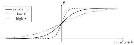
There are several other techniques for preventing over fitting that we’ll see throughout the course, e.g., data augmentation. One such technique is temperature scaling that can be applied post-hoc. Here we introduce a temperature parameter \(\tau > 0\) to the logistic function,
The effect of \(\tau\) is shown in Figure 11. A high value of \(\tau\) has a similar affect to regularization, tending to flatten the curve. A value of \(\tau\) less than one will sharpen the curve.
2.1.1 Logistic Regression as a Single Neuron
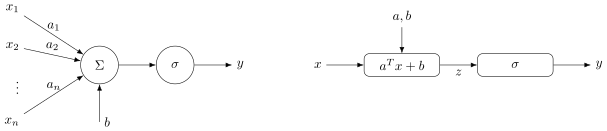
A very naive model of a biological neuron in the brain is a cell that fires its output if its accumulated input exceeds some threshold. We can very roughly view logistic regression as a single artificial neuron, as shown in Figure 12(left). The output \(y\) will be high if the weighted sum of the inputs \(z = a^Tx + b\) is greater than zero, and low otherwise. The arrows represent scalar signals. This is the classical depiction of a neuron in an artificial neural network, and is somewhat biologically inspired. The more modern view in deep learning is as a computation graph, illustrated more compactly in Figure 12(right). Here, the arrows can represent vector (or higher-order tensor) signals.
2.1.2 The XOR Problem and Multi-layer Perceptrons
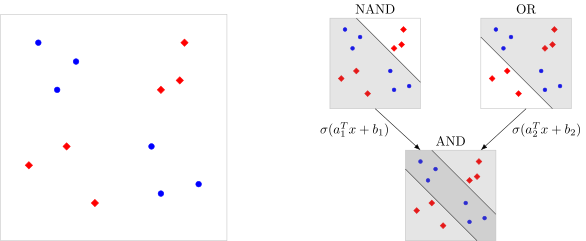
As we saw earlier, a logistic regression classifier is only able to correctly classify linearly separable data. A famous example of a problem where the data cannot be separated by a single linear decision boundary is the XOR problem. See Figure 13(left). Here examples from the positive class (blue circles) are distributed in two clusters, one close to the point \((0, 1)\) and the other close to the point \((1,0)\). Likewise, examples from the negative class (red diamonds) are distributed in two clusters, one close to the point \((1,1)\) and the other close to the point \((0,0)\). No straight line separates the two positive clusters from the two negative clusters.
The positive and negative examples can, however, be separated if we allow an additional layer of processing, as illustrated in Figure 13(right). In the first layer we construct a (linear) decision boundary \(a_1^T x + b_1\) to separate the negative cluster close to \((1,1)\) from the remaining three clusters. This can be thought of as implementing a NAND logic gate, \(\xi_1 = \sigma(a_1^T x + b_1)\), where values close to 0 map to False and values close to 1 map to True. Still in the first layer, we construct another (linear) decision boundary \(a_2^T x + b_2\) to separate the negative cluster close to \((0,0)\) from the remaining three clusters. Similar to the first decision boundary, this can be thought of as implementing an OR logic gate, \(\xi_2 = \sigma(a_2^T x + b_2)\). If we plotted \(\xi_1\) versus \(\xi_2\) we would find that the positive examples cluster around \((\xi_1, \xi_2) = (1, 1)\), whereas the negative examples cluster around either \((\xi_1, \xi_2) = (0, 1)\) or \((\xi_1, \xi_2) = (1, 0)\). As such, we can construct a second layer (linear) decision boundary \(c^T z + d\), which acts as an AND logic gate on the first layer’s output \(z = (\xi_1, \xi_2)\) to solve the XOR problem.
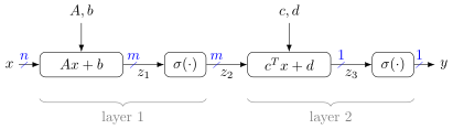
In the preceding example the first layer of processing defines new features for the second layer. This motivates the multi-layer perceptron [88, 105]. More formally, a multi-layer perceptron is defined by composing multiple layers of logistic functions. For example, a two-layer perceptron is the composed function
with parameters \(A \in \reals^{m \times n}\), \(b \in \reals^m\), \(c \in \reals^m\), and \(d \in \reals\), and where the logistic function \(\sigma\) is applied elementwise on \(z_1 = Ax + b \in \reals^m\). Parameters of multi-layer perceptrons (and other linear layers in deep learning) are often called weights. Figure 14 shows a graphical depiction of the two-layer perceptron.
To see concretely how the two-dimensional XOR problem fits the multi-layer perceptron formulation, observe that we can stack the parameters from the two neurons from the first layer as
giving
2.1.3 Activation Functions
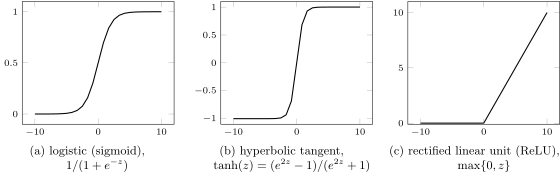
Thus far we have only considered the logistic function as operating on linear combinations of the input features. The effect of the logistic function is to produce an elementwise non-linear transformation of the features. Transformations other than the logistic function are also possible. These go under the collective name of activation functions. Other common activation functions include the hyperbolic tangent function,
and the rectified linear unit (ReLU),
These activation functions are plotted in Figure 15. For obvious reasons quantities \(z = Ax + b\) and \(y = \sigma(z)\) are often termed pre-activations and post-activations, respectively, on input \(x\). Many other activation functions have been proposed in the literature, e.g., leaky ReLU, gated linear units (GLU), GELU, SELU, radial basis, sinusoidal, etc.