Section 2.3
Multi-class and Multi-label Classification
We now extend our discussion from binary classification to multi-class and multi-label classification. In multi-class or \(K\)-way classification we are interested in assigning one label out of a predefined discrete set to each data instance, such image classification on the ImageNet dataset. For this task we are given a set of training examples \(\cD = \{(x^{(i)}, y^{(i))}\}_{i=1}^{N}\) composed of features \(x^{(i)} \in \reals^n\) and target labels \(y^{(i)} \in \{1, \ldots, K\}\). Note that while the target labels are often expressed as integers for compactness, they map to semantic categories such as dog, cat or duck. Another popular encoding is one-hot encoding where the targets are represented by a \(K\)-length vector with a one for the element associated with the class and zeros elsewhere, e.g., \((1,0,0)\) for dog, \((0,1,0)\) for cat, etc. Be aware that authors are often sloppy and the encodings are used interchangeably so that \(y^{(i)}\) is sometimes an integer and sometimes a one-hot encoding depending on the context.
We can extend the logistic function to the multi-class logistic,
parametrized by \(\{(a_k, b_k) \mid k = 1, \ldots, K\}\). The function that takes a vector \(z = (z_1, \ldots, z_K) \in \reals^{K}\) and returns \(\left(\frac{\exp z_1}{Z}, \ldots, \frac{\exp z_K}{Z}\right)\) with \(Z = \sum_{k=1}^{K} \exp z_k\) is called softmax and the \(z_k\) are called logits. The variable \(Z\) is called the partition function in machine learning and ensures that the output vector sums to one. In the context of the multi-class logistic we have \(z_k = a_k^T x + b_k\). Softmax has the property that \(\argmax_k \left\{ \frac{\exp z_k}{Z} \right\} = \argmax_k \{ z_k \}\), i.e., the index of the component that maximizes softmax is the largest logit. This means that when we want to use the model to make predictions (rather than estimate probabilities) then we can simply take the most likely prediction as the label corresponding to the largest logit.
If instead of restricting a data instance to just one label, we allowed the instance to take a set of labels, then the task becomes a multi-label classification problem. This is the same as having a set of \(K\) binary classification problems, and is typical of tasks like attribute classification. Once again we are given a set of training examples, \(\cD = \{(x^{(i)}, y^{(i))}\}_{i=1}^{N}\), composed of features \(x^{(i)} \in \reals^n\), but now the target labels are binary vectors, \(y^{(i)} \in \{0, 1\}^K\) indicating true or false for each of the categories. We model the problem using a set of \(K\) sigmoid functions,
parametrized by \(\{(a_k, b_k) \mid k = 1, \ldots, K\}\).
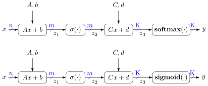
Both multi-class and multi-label problems can be solved using multi-layer perceptrons where the only difference is the final activation function, i.e., softmax or sigmoid. With parameters \(A \in \reals^{m \times n}\), \(b \in \reals^m\), \(C \in \reals^{K \times m}\), and \(d \in \reals^K\), we can write,
and depict graphically as shown in Figure 17.
There are several options for loss functions that train the models. Remember it is the loss function that tells the optimizer what to do and is a function of the model’s parameters, collectively denoted by \(\theta\) in the sequel. Unfortunately, the thing that we really care about, e.g., reducing the number of misclassified training examples, is not translatable into a loss that’s easily optimized. Specifically, we seek a loss function that is differentiable. As such, a surrogate loss function is used.
The loss function that counts the number of misclassified examples is called the 0-1 loss. It can be expressed mathematically as,
but as mentioned above it is non-differentiable so difficult to optimize.
Standard loss functions that are differentiable are mean square error (MSE),
for regression problems, and negative log-likelihood (NLL),
for classification problems. The latter is often called cross entropy loss when the probability is modeled by a multi-class logistic,
or binary cross entropy loss when applied to \(K\) independent binary variables such as for multi-label problems,
Note that all these loss functions decompose as a summation over training examples, \((x, y) \sim \cD\).
2.3.1 Aside: Treating Binary Classification as Multi-class Classification
At first glance there appears to be a discrepancy between our model for binary classification with labels \(\{0, 1\}\) and output probability defined by
and a multi-class model for the case of \(K = 2\), i.e., where we have just two labels \(\{1, 2\}\),
In the first model we have parameters \(a \in \reals^n\) and \(b \in \reals\), while in the second model we have parameters \(a_1, a_2 \in \reals^n\) and \(b_1, b_2 \in \reals\). The latter is an example of an over-parameterized model. Multiplying each of the multi-class equations by \(\frac{\exp(-a_2^T x - b_2)}{\exp(-a_2^T x - b_2)} = 1\), we get
which has the same form, and therefore the same model, as for binary classification by setting \(a = a_1 - a_2\) and \(b = b_1 - b_2\).