Section 2.4
Gradient Descent Optimization

We now turn our attention to the algorithm used to optimize the loss function—gradient descent. Let us begin by reviewing the definition of a gradient from multi-variate calculus. Let \(f : \reals^n \rightarrow \reals\) be some function, fix some \(x \in \reals^n\), and consider the expression

where \(e_i = (0, \ldots, 1, 0, \ldots)\) is the \(i\)-th canonical vector. If the limit exists, it is called the \(i\)-th partial derivative of \(f\) at \(x\) and denoted by \(\frac{\partial f(x)}{\partial x_{i}}\). The gradient of \(f(x)\) with respect to \(x \in \reals^n\) is the vector of partial derivatives,

In practice, we take derivatives using rules from calculus rather than explicitly evaluating the limits.

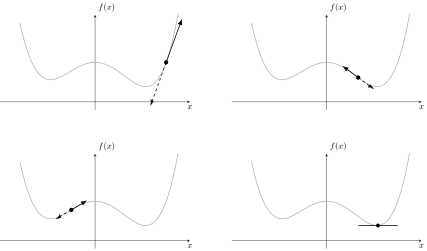
Figure 18 shows an example one-dimensional function. Several points on the function are highlighted, and the gradient at those points depicted by a solid arrow. The function decreases in the negative gradient direction. This is always true unless the gradient is zero (depicted by a horizontal line in the figure), which will occur at local maxima, local minima and saddle points. We can make use of this property to optimize the function.

The gradient descent algorithm is an iterative algorithm that takes steps in the negative gradient direction (of the loss function with respect to parameters) to seek a (local) minimum for the function. It works for smooth functions with any number of parameters. The steps can be expressed mathematically as,

where \(\eta\) is the (iteration dependent) step size or step length or learning rate that controls how big a change is made to the parameters during each iteration. Taking too big a step (i.e., very large \(\eta\)) may result in overshooting the minimum, whereas taking too small a step may result in very slow progress. Ideally, \(\eta\) is chosen by searching along the negative gradient direction for a minimum value of the function, but this is expensive to do, amounting to solving a one-dimensional optimization problem. So instead of finding the best \(\eta\), in deep learning we resort to choosing \(\eta\) via a fixed learning rate schedule.

Pseudo-code for the gradient descent algorithm is shown below:

def gradient_descent(loss, theta0):
    """Generic gradient descent method."""

    theta = theta0
    for t in range(max_iters):
        dtheta = -1.0 * gradient(loss, theta)   # descent direction is negative gradient
        eta = line_search(loss, theta, dtheta)  # choose step size by line search
        theta = theta + eta * dtheta            # update

    if (converged()):                           # check stopping criteria
        break

    return theta

The algorithm terminates when some stopping criterion is obtained, usually of the form \(\|\nabla \ell(\theta)\|_2 \leq \epsilon\), or when a maximum number of iterations is reached.

Gradient descent is very simple, we just need the gradient of the loss \(\ell\) with respect to the parameters \(\theta\) at each iteration. However, it can be very slow in its vanilla form. In later lectures we will discuss methods used in deep learning to speed up the algorithm.

The following code shows what gradient descent code looks like in PyTorch.

dataloader = ...    # way of loading batches of input-label pairs for training
model = ...         # definition of our prediction function

criterion = torch.nn.CrossEntropyLoss(reduction='mean')
optimizer = torch.optim.SGD(model.parameters(), lr=0.01)

for epoch in range(max_epochs):
    for iteration, batch in enumerate(dataloader, 0):
        inputs, labels = batch

        # zero gradient buffers
        optimizer.zero_grad()

        # compute model outputs for given inputs
        outputs = model(inputs)

        # compute and print the loss
        loss = criterion(outputs, labels)
        print(loss.item())

        # compute gradient of the loss wrt model parameters
        loss.backward()

        # take a gradient step
        optimizer.step()

The code starts with some routines for loading the data, defining the model, specifying the criterion or objective function, which is the cross entropy loss in this case, and choosing the optimization algorithm (Lines 1–5). The code the enters the optimization loop (Lines 7–25) where is processes data in batches. We will discuss the mechanics of epochs (once through the dataset) and iterations (one gradient update step) in the next lecture. For now it is sufficient to understand that each iteration the code zeros out the memory used to store gradients (Line 12), computes the models output from its input (Line 15), and calculates the loss by comparing the model’s output to the desired or target output (Line 18). This is called the forward pass. It then computes all necessary gradients via a so-called backward pass (Line 22). These gradients are accumulated into buffers associated with the model parameters, which is why it is important to zero out these buffers at the start of the loop. Last, the code updates the model parameters by taking a gradient step (Line 25).

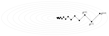
A simple example of gradient descent from Boyd and Vandenberghe [10], that also demonstrated why it can be slow, is illustrated in Figure 19. In this example we are optimizing the function,

over a two-dimensional variable \(\theta \in \reals^2\). The constant \(\gamma\) gives us a family of functions. We start at \(\theta^{(0)} = (\gamma, 1)\) and use exact line search. This allows us to calculate the iterates determined by the gradient descent algorithm in closed-form:

Note that convergence will be very slow if \(\gamma \gg 1\) or \(\gamma \ll 1\). In the figure we use \(\gamma = 10\).

One question remains: how do we calculate the gradients? To finish the lecture we give a worked example for the two-layer perceptron with logistic activation functions. In the next lecture we will discuss gradient calculation for deep learning in much more detail and introduce automatic methods for performing the calculations for us. Nevertheless, it is a valuable exercise to work through computing gradients by hand at least once.

Consider the two-layer perceptron expressed as

where \(\sigma(\xi) = (1 + e^{-\xi})^{-1}\) is applied elementwise. We will assume an arbitrary differentiable loss function \(\ell\) that we wish to minimize. As such, we can assume that \(\fracdd[\ell]{y}\) is given. But we need to compute gradients of the loss for all of our parameters, i.e., \(\fracdd[\ell]{A}\), \(\fracdd[\ell]{b}\), \(\fracdd[\ell]{c}\) and \(\fracdd[\ell]{d}\), so that we can perform gradient descent.

First, observe that

Starting at the second layer, let \(\xi = c^T z + d\). We have, by the chain rule of differentiation,

since \(\fracdd[y]{\xi} = y(1 - y)\) by our observation and \(\fracdd[\xi]{d} = \fracdd[c^Tz + d]{d} = 1\), and

where in the last line we, again, used the fact that \(y = \sigma(\xi)\) and \(\nabla_c \xi = \nabla_c (c^T z + d) = z\).

Moving backward onto the first layer, we have

following the same pattern as \(\nabla_{\!c} \ell\). Then, for the first layer’s parameters,

where \(\circ\) denotes elementwise product. These expressions use vector operations and can be a little intimidating when seen for the first time. If you find these difficult to interpret, try computing gradients on individual parameters using only scalar-valued derivatives, e.g.,

where \(z_k = [\sigma(Ax + b)]_k = \sigma(\sum_{p} A_{kp} x_p + b_k)\) and noting that \(\fracdd[z_k]{A_{ij}} = 0\) if \(k \neq i\). When \(k = i\) we have,

so completing the derivative by substituting for all \(\fracdd{\cdot}\) terms we get

Notice that we have reused calculations from evaluation of \(\ell\), i.e., \(y\) and \(z\), in our expressions for the gradients. We could just have legitimately written the gradients in terms of the input \(x\) only. How we write these expressions leads to an important consideration of memory-vs-compute trade-off that will be discussed in later lectures. Stay tuned.