Section 3.2
Automatic Differentiation
Automatic differentiation (AD) is an algorithmic procedure that produces code for computing exact derivatives (up to machine precision). This is in contrast to numerical methods for estimating gradients such as with finite differences. The approach assumes that all calculations are composed from a small set of elementary operations that we know how to differentiate, e.g., arithmetic operations, exponentiation, logarithms, and trigonometric functions.
It is not an exaggeration to say that modern deep learning would not be possible without automatic differentiation—it greatly reduces development and testing effort, and allows for rapid prototyping of new ideas.
Automatic differentiation comes in two flavours. Forward mode automatic differentiation fixes an independent variable \(u\) and computes derivatives \(\fracdd[v]{u}\) for all dependent variables \(v\). In contrast, reverse mode automatic differentiation fixes a dependent variable \(v\) and computes derivatives \(\fracdd[v]{u}\) for all independent variables \(u\).
Consider the simple three-node network below, where a loss function \(L\) is computed on the output \(y\), itself a function of the input \(x\) and parameters \(\theta_1\), \(\theta_2\) and \(\theta_3\),
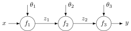
The chain rule of differentiation allows us to write the derivative of the loss with respect to parameter \(\theta_1\) as,
Forward mode automatic differentiation evaluates this expression from right to left, first computing \(\fracdd[z_2]{\theta_1} = \fracdd[z_2]{z_1} \fracdd[z_1]{\theta_1}\), then \(\fracdd[y]{\theta_1} = \fracdd[y]{z_2} \fracdd[z_2]{\theta_1}\), and finally \(\fracdd[L]{\theta_1} = \fracdd[L]{y} \fracdd[y]{\theta_1}\),
so by the end we have computed \(\fracdd[v]{\theta_1}\) for all variables \(v \in \{z_1, z_2, y, L\}\).
Reverse mode automatic differentiation evaluates the other way around, i.e., from left to right,
so that by the end of the calculation we have computed \(\fracdd[L]{u}\) for all variables \(u \in \{y, z_2, z_1, \theta_1\}\).
3.2.1 Dual Numbers for Forward Mode AD
A useful representation for computing forward mode automatic gradients on-the-fly is the dual number representation. Here each variable \(v\) is replaced with \(v + \Delta v\), where \(\Delta v\) represents an infinitesimal change in \(v\). As such, quantity \(\Delta v\) has the property that \((\Delta v)^2 = 0\). Setting \(\Delta u = 1\) for an independent variable \(u\) and then computing all dependent variables will result in \(\Delta v = \fracdd[v]{u}\). We illustrate this with three examples.
Example 1. In this first example we show how to compute gradients with dual numbers for the affine transformation \(y = ax + b\),
which for \(\Delta x = 1\) gives the expected result \(\fracdd[y]{x} = a\).
Example 2. Next we look at the more complicated example of \(y = \exp(x)\). Here we first expand the exponential function into its infinite polynomial series, \(\exp(x) = \prod_{n=0}^{\infty} \frac{x^n}{n!}\), so that we can write,
where in Line \(\ref{eqn:dual_num_grouping}\) we have grouped together terms involving \(\Delta x\) (all higher-order terms of \(\Delta x\) having been dropped using the property that \(\Delta x^2 = 0\)), and then in the following line replaced the infinite series with the corresponding \(\exp(x)\) terms. Once again setting \(\Delta x = 1\) we arrive at \(\fracdd[y]{x} = \exp(x)\) as expected.
Example 3. Last, let us compute the gradient of \(y = 1/x\),
giving \(\fracdd[y]{x} = -1/x^2\). These three examples are all we need for computing the gradients necessary for MLP training.
3.2.2 Cost of Gradient Evaluation Ordering
In training deep learning models we usually want to update all parameters at the same time. Consider the simple three-node deep learning model from earlier, reproduced below with the size of the intermediate variables annotated,
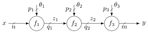
and with parameters \(\theta = (\theta_1, \theta_2, \theta_3)\) of total size \(p = p_1 + p_2 + p_3\). Both forward and reverse mode automatic differentiation compute the quantity,
Focusing on the first term we have,
where we have written the size of each gradient matrix under it in the expression.
Forward mode automatic differentiation evaluates the expression from the right, first computing \(\fracdd[z_2]{\theta_1} = \fracdd[z_2]{z_1} \fracdd[z_1]{\theta_1}\) of size \(q_2\)-by-\(p_1\), then \(\fracdd[y]{\theta_1} = \fracdd[y]{z_2} \fracdd[z_2]{\theta_1}\) of size \(m\)-by-\(p_1\), and finally \(\fracdd[L]{\theta_1} = \fracdd[L]{y} \fracdd[y]{\theta_1}\) of size 1-by-\(p_1\). The total computational cost is therefore,
Reverse mode automatic differentiation on the other hand evaluates the expression from the left, first computing \(\fracdd[L]{z_2} = \fracdd[L]{y} \fracdd[y]{z_2}\) of size 1-by-\(q_2\), then \(\fracdd[L]{z_1} = \fracdd[L]{z_2} \fracdd[z_2]{z_1}\) of size 1-by-\(q_1\), and finally \(\fracdd[L]{\theta_1} = \fracdd[L]{z_1} \fracdd[z_1]{\theta_1}\) of size 1-by-\(p_1\). The total computation cost for reverse mode is therefore,
which can be significantly faster than the forward mode.
The operations for computing intermediate terms during reverse mode automatic differentiation are often called vector-Jacobian products for obvious reasons—we are always multiplying the gradient of the loss, which is a vector, by a so-called Jacobian matrix. This is generally much more efficient in deep learning where the function we are differentiating, i.e., \(L\), is scalar-valued and there are a large number of parameters \(\theta\).