Section 3.4
Putting it all Together

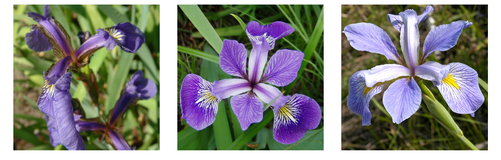
Let’s put what we have learned so far together to build an flower classifier. We won’t be extracting features directly from images but rather making use of an existing dataset where features of example flowers have already been measured for us manually. The dataset is the Iris dataset collected by the famous statistician Sir Roland Fisher in 1936. It contains 150 examples of Iris flowers. The flowers are divided into three classes—Setosa, Versicolour, and Virginica—with 50 examples per class. Each example is characterized by a 4-dimensional feature vector representing the flower’s sepal length, sepal width, petal length and petal width. Examples of the different classes is shown in Figure 24.

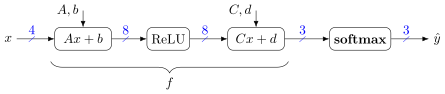
Figure 24: The Iris dataset (Fisher, 1936) is a small classical dataset used to develop and evaluate classification algorithms. It consists of 150 examples of three different classes of Iris flower—Setosa, Versicolour, and Virginica. Each instances has four features measuring properties of the flower.

The existence of the pre-measured features significantly simplifies the problem. Nevertheless, it will make for an instructive case study based on what we have learned thus far in the course. To classify examples we will train a multi-layer perceptron with four inputs, eight hidden nodes with ReLU activation function, and three outputs normalized by softmax. The model architecture, which should be quite familiar to you by now, is shown below.

The parameters of the model, \(\theta = \{A, b, C, d\}\), will be tuned using gradient descent with cross-entropy loss,

\begin{align} \ell(\theta; x, y) &= -\log \left[\textbf{softmax}(f(x; \theta))\right]_y. \tag{117}\end{align}

Here, \(\left[\cdot\right]_y\) indicates taking the entry from \(\textbf{softmax}(f(x; \theta))\) corresponding to the ground-truth label \(y\). In this case study we will use all 150 examples as our training data, so the loss \(L\) is summed over the entire dataset,

\begin{align} L(\theta) &= \sum_{i=1}^{150} \ell(\theta; x^{(i)}, y^{(i)}) \tag{118}\end{align}

with gradient updates,

\begin{align} \theta \gets \theta - \eta \nabla L(\theta). \tag{119}\end{align}

However, for real applications it is better to split the data into training, validation and test subsets, and only update the parameters based on the training subset. We will discuss the reason for doing this later in the lecture.

PyTorch’s nn.CrossEntropyLoss function computes softmax internally so we can removed it from the software implementation of our model. This does not matter for prediction since taking the maximum element after the softmax is the same as taking the maximum element before softmax (i.e., on the logits).

There are two ways to implement our multi-layer perceptron in PyTorch. Since the model is a simple chain of processing nodes we can defined it using the nn.Sequential container. This container takes a list of nodes (also called modules in PyTorch) and connects the output of each node to the input of the next node in the sequence.

model = nn.Sequential(
    nn.Linear(4, 8, bias=True),
    nn.ReLU(True),
    nn.Linear(8, 3, bias=True)
)

The second way to implement our model is by specializing the nn.Module class. This is much more flexible in that arbitrary processing can be performed within the forward method. Here we simply compute the output of each layer in turn using as input the output from the previous layer. Layers are instantiated in the __init__ method. Finally, on Line 18 we create an object of the multi-layer perceptron class.

class IrisMLP(nn.Module):
    """Multi-layer perceptron for Iris Dataset."""

    def __init__(self):
        super().__init__()

        self.layer1 = nn.Linear(4, 8, bias=True)
        self.layer2 = nn.ReLU(True)
        self.layer3 = nn.Linear(8, 3, bias=True)

    def forward(self, x):
        z1 = self.layer1(x)
        z2 = self.layer2(z1)
        y_hat = self.layer3(z2)

    return y_hat

model = IrisMLP()

In both ways of implementing the model, the trainable parameters are automatically created and initialized as part of the nn.Linear layers. But what values are the parameters initialized to? Remember that we wish to avoid vanishing and exploding gradients. Therefore it makes sense to initialize the parameters so that the activation functions are operating in their linear region. For the logistic function this is around zero.

One good approach is to randomly draw parameter values i.i.d. from a zero-centered Gaussian, \({\cal N}(0, \sigma^2)\), or symmetric uniform distribution, \({\cal U}(-\sigma, \sigma)\), where \(\sigma\) is small. The bias terms, \(b\) and \(d\) are typically set to zero. More sophisticated approaches consider the fan-in and fan-out of a node to try control the variance of the features as the propagate through the network. Two popular options are Golorot or Xavier initialization [31], which sets the Gaussian standard deviation as

\begin{align} \sigma &= \sqrt{\frac{2}{n_i + n_o}} \tag{120}\end{align}

where \(n_i\) and \(n_o\) are the number of inputs and number of outputs, respectively, and Kaiming initialization [40], which sets

\begin{align} \sigma = \sqrt{\frac{2}{n_i}} \quad \text{ or } \quad \sigma = \sqrt{\frac{2}{n_o}} \tag{121}\end{align}

to work better for models with ReLU activation functions.

Some tasks require more specialized initialization techniques to guide training towards particular solutions or away from degenerate ones. The spherical initialization for 3D shape fitting [9] is a good example of such techniques.

3.4.1 Training

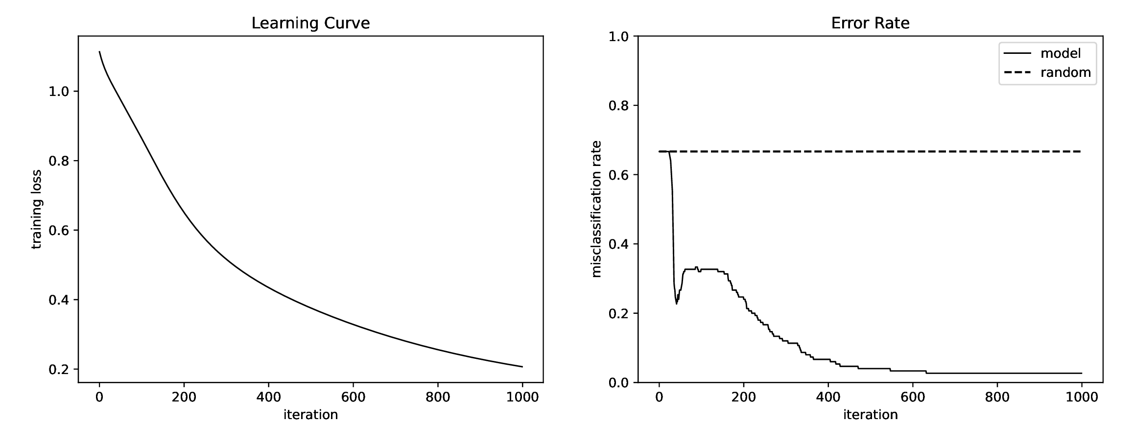
Once we start training our model we want to keep track of how well the model is doing. Learning curves are a good way of doing this by plotting the training loss (or any other performance metric) as a function of training iteration. An example for training our Iris classification model is shown in Figure 25. Notice that the training loss decreases steadily with number of iterations. The second plot shows how misclassification or error rate changes as the model is trained. Randomly guessing would result in an error rate of \(\frac{2}{3}\), since we have a balanced three-class problem. This is where the model starts when it is initialized. As the model trains the number of errors tends towards zero, but not necessarily in a monotonic way.

It can be mesmerizing to watch the learning curves as your model trains. And while learning curves are very helpful in diagnosing problems early, many a researcher has wasted hours and hours enjoying the peace and quiet of just staring at learning curves. This is something to be avoided.

You will often hear the term learning dynamics or optimization dynamics to describe the patterns and behaviours exposed by learning curves. Understanding these dynamics can sometimes help improve the design of learning algorithms as we will see throughout the remainder of this lecture.

Figure 25: Learning curves plot performance metrics as a function of training iteration. They are very useful for diagnosing problems with your model or training algorithm.

Our task for Iris classification in this case study is small and the full training dataset can be easily processed to calculate the gradient at each iteration. However, for big models (e.g., ImageNet), using the entire dataset to calculate the gradient is very expensive. Recall that many loss functions decompose over training data \(\{(x^{(i)}, y^{(i)})\}_{i=1}^N\), and hence so does the gradient. Thus far we have not been concerned with scaling factors, but in practice the loss function is normalized by the size of the training dataset \(N\), making it somewhat invariant to the amount of training data,

\begin{align} L(\theta) &= \frac{1}{N} \sum_{i=1}^{N} \ell(f(x^{(i)}; \theta), y^{(i)}) \tag{122}\end{align}

giving the gradient as

\begin{align} \nabla_\theta L(\theta) &= \frac{1}{N} \sum_{i=1}^{N} \nabla_\theta \, \ell(f(x^{(i)}; \theta), y^{(i)}) \tag{123}\end{align}

Stochastic gradient descent (SGD) is a method for approximating gradients by using only a subset of the data, called a mini-batch, \(\cI \subseteq \{1, \ldots, N\}\), to get

\begin{align} \widehat{\nabla_\theta L} &= \frac{1}{|\cI|} \sum_{i \in \cI} \nabla_\theta \, \ell(f(x^{(i)}; \theta), y^{(i)}) \tag{124}\end{align}

The number of training examples in \(\cI\) is called the batch size.

Under mild assumptions the expected value of the approximate gradient from stochastic gradient descent will equal the true gradient, i.e., \(E [ \widehat{\nabla_\theta L} ] = \nabla_\theta L\). This is good news because it means that over a large number of training iterations stochastic gradient descent will behave the same as gradient descent, and each iteration can be performed much, much faster. Gradients can also be accumulated over multiple mini-batches for a better estimate of the immediate gradient, which is sometimes done in a distributed fashion making use of parallel compute.

In practice we shuffle the indices of examples in the training dataset, i.e., we randomly permute \([N]\), and iterate through adjacent fixed-length intervals. Under this regime each gradient update step is called an iteration, and once through the dataset is called an epoch. The dataset is reshuffled at the start of each epoch to avoid biasing the model to perform well on just the last mini-batch in the shuffled dataset.

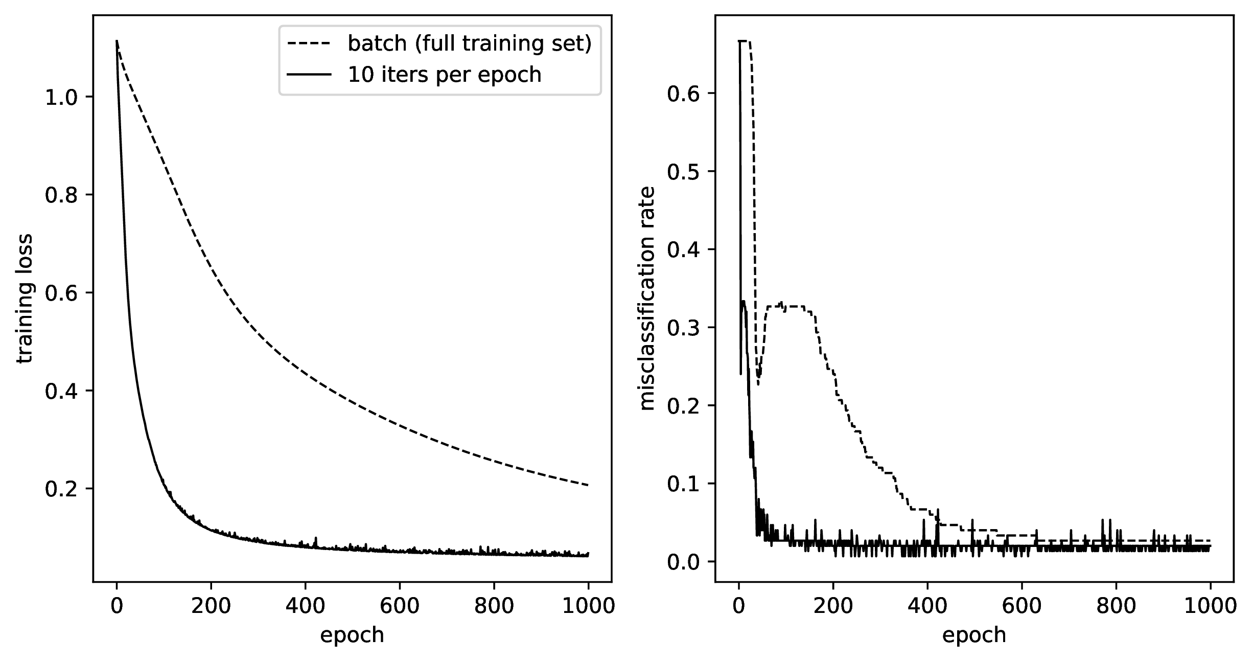
Figure 26 shows learning curves comparing stochastic gradient descent with gradient descent for our Iris classification problem. For the stochastic setting we choose a mini-batch size of 15, so it takes 10 iterations to complete an epoch. Notice that despite a noisy gradient estimate, here stochastic gradient descent converges much faster, although this is not always the case.

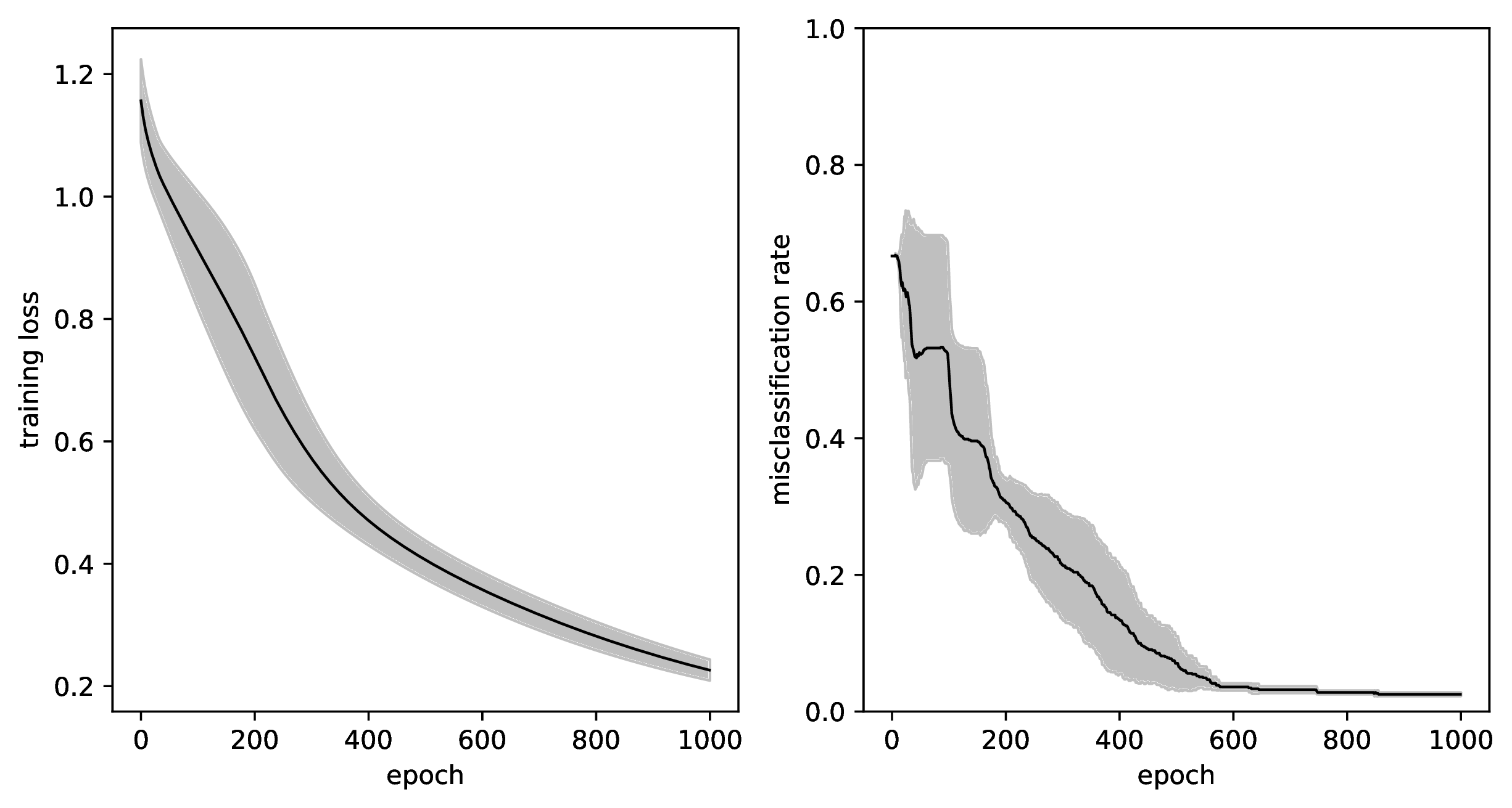
Deep learning models are generally non-convex functions so different parameter initializations and different mini-batch orderings may produce different results. Even different hardware and software libraries can cause differences in training, due to accumulation of small numerical differences or race conditions in the hardware. It is important when comparing methods that any perceived improvement is not a result of a lucky random seed favouring one method over another. Figure 27 shows the average learning curve over five training runs initialized with different random seeds. The shaded area shows one standard deviation of performance (measured at each iteration). In this simple example the five runs converge to the same final error rate.

Figure 27: Different random parameter initializations can result in different learning curves. Shown is the mean and one standard deviation over five training runs, each with a different random seed.

One of the most important questions in deep learning is which model to deploy? Taking the model defined by the parameters from the last training iteration is not always the best since deep learning is prone to overfitting. Standard practice it to break the dataset into three disjoint subsets, each playing a different role. First, the training set is used for estimating gradients and updating the model parameters. Second, the validation set is used for selecting the model (i.e., set of parameters) to deploy. Every epoch or so during training the model parameters can be saved so that the model can be evaluated or have further diagnostics run later. This is known as check-pointing. The third subset, known as the test set, is used to evaluate generalization performance on the model chosen by the validation set. Ideally, the test set is never seen by model developers to avoid inadvertently using it to tweak model performance and therefore provide an invalid estimate of how it will perform on new data when deployed.

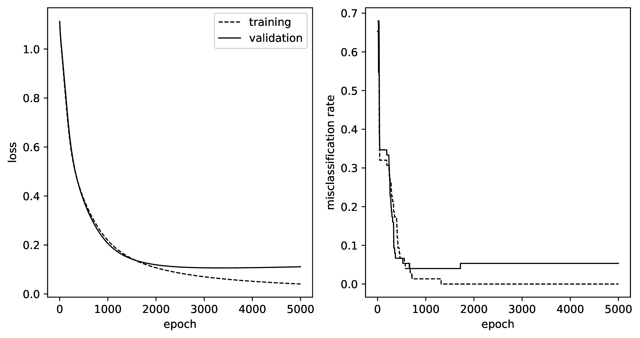
Figure 28 shows learning curves for the Iris classifier on a training subset and validation subset. Here we randomly shuffle the data and use the first half for training and second half for validation. That is, only 75 examples are used to estimate the gradient of the loss and update model parameters. The other 75 examples are used to track performance. Notice that as training proceeds the model does better on the training subset than the validation subset. This is a classic case of overfitting. In this example we would deploy the model parameters obtained at around 1000 training iterations rather than the model which achieves lowest training loss (at 5000 iterations).

Figure 28: Training set versus validation set performance. Here we randomly shuffled the Iris dataset, and used the first half (75 examples) for training and second half (75 examples) for validation.

There are several mechanisms that can be used to improve generalization performance. These include adding an explicit regularization term to the loss function, which is very standard in machine learning as we have already seen. We can also implicitly regularize the parameters through data augmentation. This is a technique that adds random noise/perturbations to the input data in an attempt to force the model to deal with slight variations of the training data that is may see at test time. Data augmentation is very standard in deep learning and built into the training pipelines of deep learning software frameworks. We’ll be looking at some specific data augmentation approaches designed for computer vision applications in later lectures.

Another option is to collect more real training data. This is evident in the massive influence the large-scale ImageNet dataset had in solving the image classification problem. Unfortunately, this can also be very expensive and in some applications may not be possible (e.g., medical imaging or data from the surface of Mars).

The last mechanism, which has had surprising success in deep learning, is to use large-scale generic pre-training, on a dataset such as ImageNet, followed by finetuning on a smaller dataset curated for the specific task. Here finetuning refers to continued training of the model on the task-specific data, and can be thought of as a type of transfer learning.

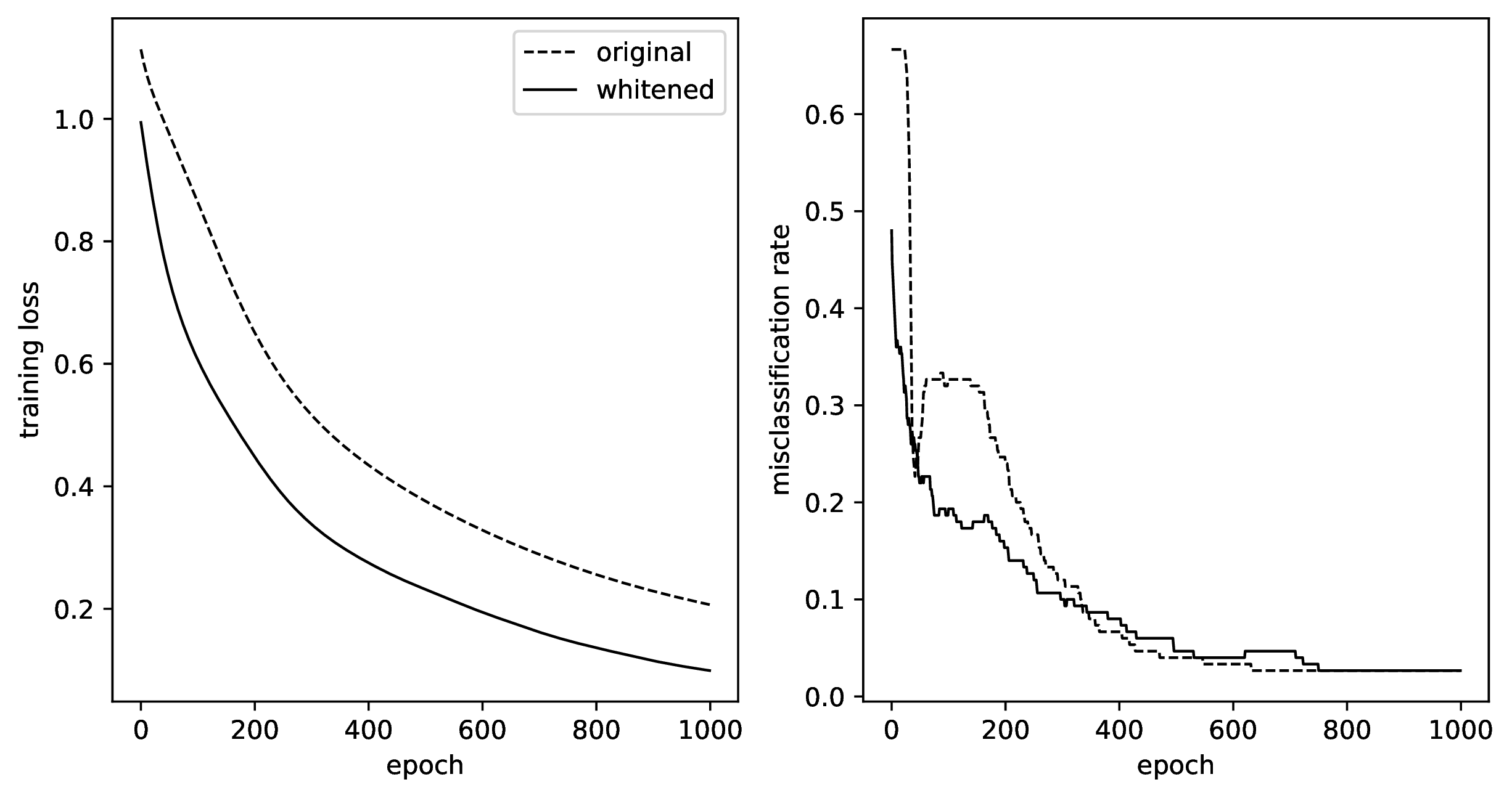
The scale and distribution of features can have a big impact on training and model performance. We saw this in the example gradient descent optimization example in Figure 19 from the last lecture. Normalizing, also known as whitening, the data to have zero mean and unit covariance often improves convergence and generalizability as shown in Figure 29. Mathematically we have,

\begin{align} x^{(i)} &\gets \Sigma^{-1} (x^{(i)} - \mu), & \text{for $i = 1, \ldots, N$} \tag{125}\end{align}

where \(\mu\) and \(\Sigma\) are the feature mean and covariance over the training dataset.

On large-scale data it is impractical to compute the full covariance matrix \(\Sigma\) so we typically normalize each dimension of the data independently,

\begin{align} x^{(i)}_j &\gets \frac{x^{(i)}_j - \mu_j}{\sigma_j}, & \text{for $j = 1, \ldots, n$} \tag{126}\end{align}

where \(\mu_j\) is the mean of the \(j\)-th feature over the training data, and \(\sigma_j\) is its standard deviation. When applied to features within a deep learning model from online estimates of the mean and standard deviation, this is called batch normalization (or BatchNorm) and will be discussed in later lectures.

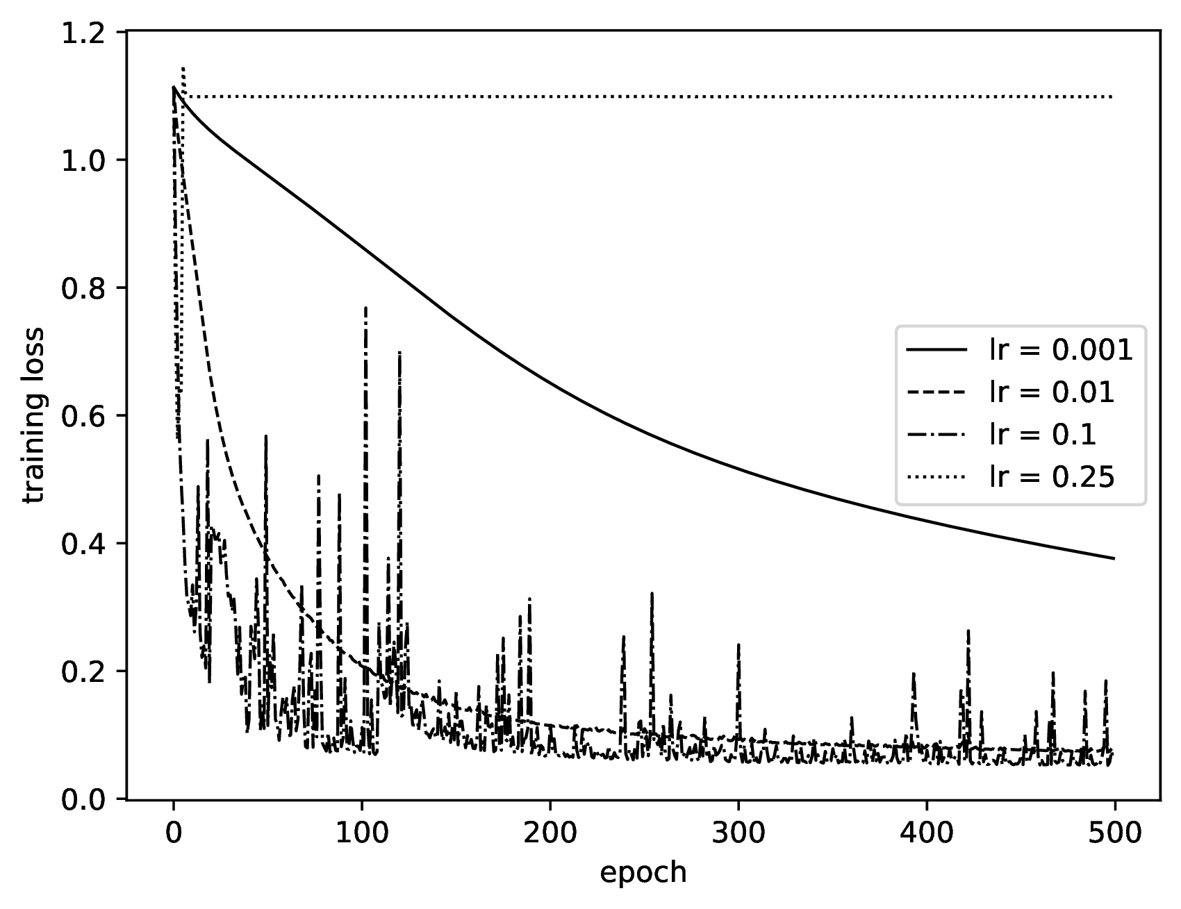
Figure 29: Normalizing data, also called whitening, often improves training convergence and stability. The learning rate here has been rescaled based on the average feature magnitude.

The learning rate \(\eta\) is an example of a hyperparameter and its value can also have a big influence on performance and convergence rate. Figure 30 shows learning curves for training our Iris classification model with different learning rates. As evident in the figure, too small a learning rate results in very slow convergence, whereas too large a learning rate can lead to unstable training and can even get the model stuck.

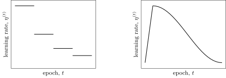
We do not need to use the same learning rate each epoch, and experience has shown that varying the learning rate can have a significant effect on training. A rule for determining the learning rate at each epoch is called a learning rate schedule. So far we have only considered a constant learning rate, \(\eta^{(t)} = \eta_0\). Other popular learning rate schedules include the linear schedule,

\begin{align} \eta^{(t)} &= \eta_{\text{init}} + \frac{t}{t_{\text{max}}} \left(\eta_{\text{final}} - \eta_{\text{init}} \right), \tag{127}\end{align}

the step schedule,

\begin{align} \eta^{(t)} &= \begin{cases} \gamma \eta^{(t-1)}, & \text{if $t \,\%\, t_{\text{step}} = 0$} \\ \eta^{(t-1)}, & \text{otherwise} \end{cases} \tag{128}\end{align}

and the cosine schedule,

\begin{align} \eta^{(t)} &= \eta_{\text{min}} + \frac{1}{2}\!\left(\eta_{\text{max}} - \eta_{\text{min}} \right) \left(\! 1 + \cos \left(\frac{\pi t}{t_{\text{period}}} \right) \! \right) \tag{129}\end{align}

Combinations of learning rate schedules can also be used, e.g., linear warm-up with cosine decay. Figure 31 shows this combination as well as the step learning rate schedule. A jump (rapid decrease) in training loss often accompanies a step change in the learning rate.

Learning rate, , can have a significant effect on training convergence. Too small a learning rate and convergence can be very slow, too high a learning rate res — Figure 30: Learning rate, \(\eta\), can have a significant effect on training convergence. Too small a learning rate and convergence can be very slow, too high a learning rate results in unstable training, which can sometimes get the model stuck.

Learning rate schedules, : (left) step learning rate, (right) linear warm-up followed by cosine decay — Figure 31: Learning rate schedules, \(\eta^{(t)}\): (left) step learning rate, (right) linear warm-up followed by cosine decay.

Stochastic gradient descent can still be slow even with a good learning rate schedule and whitening of the data. This prompted researchers to explore alternative pseudo-second-order schemes to improve convergence rate. One popular method is to add momentum (also called the heavy ball method),

\begin{align} g^{(t)} &= \nabla L(\theta^{(t)}) + \mu g^{(t-1)} \tag{130}\\ \theta^{(t+1)} &= \theta^{(t)} - \eta g^{(t)} \tag{131}\end{align}

which adds a multiple of the previous gradient to the current gradient estimate. This tends to smooth out any noise in the stochastic gradient estimate and keep the parameters moving in the same direction much like a heavy ball rolling down a bumpy road.

Other popular methods include AdaGrad [24], Adam [53] and AdamW [70], all of which we will discuss shortly. Each method comes with a set of hyper-parameters and you need to play around to see what works best for your problem, using the learning curves as a guide. A good strategy is to start with a method and schedule that had been demonstrated to work well for similar tasks or network architectures, and then adapt the various hyper-parameters in a process known as hyper-parameter tuning. An active area of research is exploring how to set the hyper-parameters automatically.

AdaGrad [24] is a method inspired by classical optimization algorithms. It views gradient descent as updating the parameters according to a first-order proximal method that solves the optimization problem,

\begin{align} \theta^{(t+1)} &= \argmin_{\theta} \left\{ \langle\nabla L (\theta^{(t)}), \theta\rangle + \frac{1}{2\eta_t} \|\theta - \theta^{(t)}\|_2^2 \right\} \tag{132}\end{align}

whose solution, obtained by differentiating the objective and setting to zero, is the standard gradient update,

\begin{align} \theta^{(t+1)} &= \theta^{(t)} - \eta_t \nabla L(\theta^{(t)}) \tag{133}\end{align}

As we’ve seen, however, this can lead to slow convergence because of the geometry of the loss landscape requiring different features to be scaled differently. The trick with AdaGrad is to adapt the step size (geometry) for different features to increase influence of rare but informative features by changing the norm of the proximal term in the above formulation,

\begin{align} \theta^{(t+1)} &= \argmin_{\theta} \left\{ \langle\nabla L(\theta^{(t)}), \theta\rangle + \frac{1}{2\eta_t} \|\theta - \theta^{(t)}\|_B^2 \right\} \tag{134}\end{align}

giving

\begin{align} \theta^{(t+1)} &= \theta^{(t)} - \eta_t B^{-1} \nabla L(\theta^{(t)}) \tag{135}\end{align}

The matrix \(B\) encodes the curvature of the loss landscape. In the classical Newton’s method it would be the Hessian matrix, \(\nabla^2 L(\theta^{(t)})\). However, this is too expensive to compute for large-scale problems being quadratic in the number of parameters. AdaGrad estimates \(B\) as a diagonal matrix using previous gradients,

\begin{align} G^{(t)} &= \left(\textstyle \sum_{k=1}^{t} \diag{\nabla L(\theta^{(k)})}^{\!2} + \epsilon I\right)^{\!1/2} \tag{136}\end{align}

which is only linear in the number of parameters and easily invertible. The main weakness of AdaGrad is that elements of the matrix \(G^{(t)}\) keep growing so the learning rate becomes infinitesimally small over time.

Adam [53] fixes the above problem with AdaGrad by maintaining exponentially decaying averages of past gradients and gradients-squared,

\begin{align} m^{(t)} &= \beta_1 m^{(t-1)} + (1 - \beta_1) \nabla L(\theta^{(t)}) \tag{137}\\ v^{(t)} &= \beta_2 v^{(t-1)} + (1 - \beta_2) \nabla L(\theta^{(t)})^2 \tag{138}\end{align}

To ensure an unbiased estimate (c.f. unbiased variance calculations) it modifies these decaying averages as,

\begin{align*} \hat{m}^{(t)} = \frac{1}{1 - \beta_1^t} m^{(t)} \text{ and } \hat{v}^{(t)} = \frac{1}{1 - \beta_2^t} v^{(t)} \end{align*}

The update rule according to the Adam method is then,

\begin{align} \theta^{(t+1)} &= \theta^{(t)} - \eta \, \diag{\hat{v}^{(t)} + \epsilon}^{\!-1/2} \hat{m}^{(t)} \tag{139}\end{align}

AdamW [70] goes one step further and includes weight decay within the Adam update,

\begin{align} \theta^{(t+1)} &= \theta^{(t)} - \eta \, \diag{\hat{v}^{(t)} + \epsilon}^{\!-1/2} \left(\hat{m}^{(t)} + w \theta^{(t)} \right) \tag{140}\end{align}

This has been shown empirically to work better than applying \(\ell_2\) regularization on \(m^{(t)}\) separately. AdamW is the de facto standard update rule (for now), although there are many other variants and combinations.

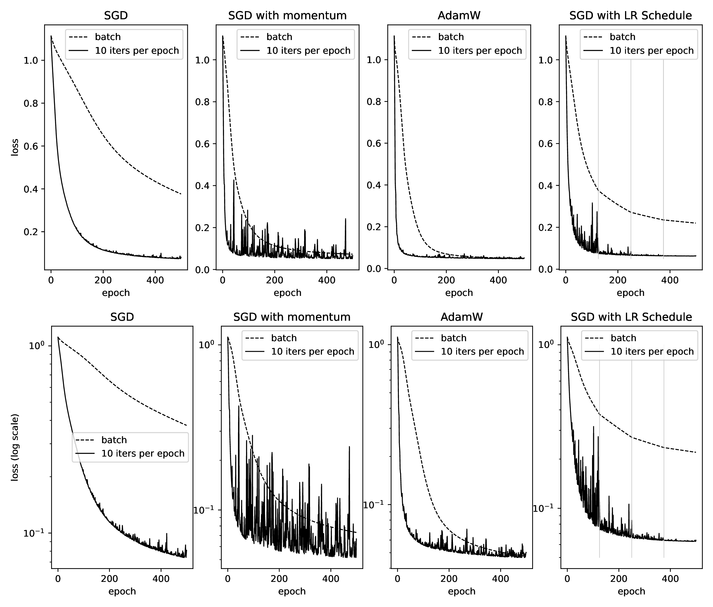
Figure 32: Comparison of learning curves for different variants of gradient descent and stochastic gradient descent. Here we plot the loss on a linear scale (top) and log scale (bottom). The latter is often more useful to see progress as training converges.

A comparison of learning curves for vanilla stochastic gradient descent (SGD), momentum, AdamW and the step learning rate schedule are show in Figure 32. SGD, momentum and AdamW use the same fixed step size whereas the step learning rate schedule starts higher and drops to lower during training. Observe that momentum accelerates convergence but can also be unstable. AdamW is overall the best for this problem.

Section 3.4Putting it all Together

3.4.1 Training

Section 3.4
Putting it all Together