Section 3.3
Back Propagation

Back-propagation is the term used in deep learning for computing gradients, essentially using reverse mode automatic differentiation together with caching of intermediate results. Different deep learning frameworks use slightly different approaches (explicit graph construction versus eager evaluation and operator tracking). But in all frameworks the developer only needs to implement the forward pass operation for a node and the backward pass is automatically generated. Conceptually, for each line of the forward pass code, P, Q = foo(A, B, C), automatic differentiation needs to produce a line dLdA, dLdB, dLdC = foo_vjp(dLdP, dLdQ) in the backward pass code. Here vjp stands for vector-Jacobian product. Usually the inputs A, B and C, and outputs P and Q are also made available to foo_vjp in the backward pass.

So, to summarize, a deep learning node (sometimes called a layer) in a deep learning network,

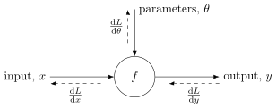
needs to implement two operations. In the forward pass the node computes the output \(y\) as a function of the input \(x\) and parameters \(\theta\). In the backward pass the node computes the derivative of the loss function with respect to the input \(x\) and the parameters \(\theta\) given the derivative of the loss with respect to the output \(y\). In PyTorch these operations appear as follows:

Let us look at a simple node that we may want to include within a deep learning model, that of computing the inverse square-root of a positive number \(x\),

This has application, for example, in 3D scene rendering where \(x\) represents the magnitude of a normal vector, and the aim is to produce a unit normal. The calculation in the forward pass is composed of elementary operations, namely square-root and inverse, and so can be automatically differentiated. Alternatively, we could provide a hand-coded implementation of the derivative. We have,

So in the backward pass, given \(\ifracdd[L]{y}\), the node would compute,

Notice that we have chosen to use the output of the node, \(y\), in the implementation of the expression for the gradient in the backward pass. This requires storing the value in the forward pass for re-use later on, and is a typical pattern in deep learning frameworks. In this example, we could also have implemented the backward pass in terms of \(x\), but that would have required taking its square-root a second time.

3.3.1 Batched Operations

Consider an abstract deep learning node with \(n\)-dimensional input \(x\), \(m\)-dimensional output \(y\), and \(p\)-dimensional parameters \(\theta\), shown here with the shape of inputs, output, and parameters annotated,

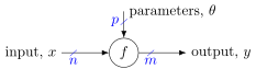
The Jacobian matrices \(\fracdd[y]{x}\) and \(\fracdd[y]{\theta}\) are (\(m\)-by-\(n\))-dimensional and (\(m\)-by-\(p\))-dimensional matrices of partial derivatives \(y\) with respect to \(x\) and \(\theta\), respectively. The gradients \(\fracdd[L]{y}\), \(\fracdd[L]{x}\) and \(\fracdd[L]{\theta}\) are a \(m\)-, \(n\)-, and \(p\)-dimensional (row) vectors, respectively. Now recall that in deep learning we process data in batches of, say, \(N\) samples. As such, the gradient quantities computed by the node in the backward pass are

and

where the shape of each term has been marked. Notice that for the input we have \(N\) independent vector-Jacobian products, whereas for the parameters we sum the vector-Jacobian products over training instances. In practice, instead of forming \(\fracdd[y]{x}\) explicitly, code can compute \(\fracdd[L]{x}\) directly from \(\fracdd[L]{y}\) if more efficient to do so.

3.3.2 Vanishing and Exploding Gradients

Training deep learning models involves evaluating long chains of gradient multiplications, e.g.,

This can result in the so-called vanishing and exploding gradient problem, i.e., successive multiplication of small numbers making the gradient go to zero, or successive multiplication of large numbers making the gradient calculation overflow.

The problem is particularly pronounced with sigmoid-like activation functions, which have flat regions, hence zero gradient, away from the origin. A great deal of effort has been devoted to developing techniques to mitigate against vanishing or exploding gradients. We will see some of these later in the lecture.

3.3.3 Memory Layout and Usage in Deep Learning

Deep learning models consume vast quantities of data to train. The data is often processed in batches to reduce computational load and memory requirements. A batch of data may have shape something like \(B \times C \times H \times W\) for a batch of size \(B\) elements of \(C\)-channel 2D features maps. An example illustrating memory layout as a batch of data is processed through a model is shown in Figure 22. Blue boxes indicate tensors in the forward pass, gray boxes indicate memory that stores model parameters, and red boxes depict gradient tensors in the backward pass. The batch size stays constant through the network but the dimensionality of the rest of the tensor may change. Parameters are not batched, they are shared across batch elements.

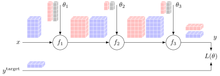
There are a few of things to observe. First, parameters only take a small amount of memory (relative to data).¹ Second, gradients take the same amount of space as the features from the forward pass. Gradients are stored transposed so that their shape exactly matches the forward pass tensor. Third, in-place operations may save memory in the forward pass. However, during training intermediate results from the forward pass may be needed to compute gradients. In-place operations must not destroy this information. Re-using memory buffers may save some memory in the backward pass, but this can be challenging to implement and of minor utility since feature size (and hence memory requirements) usually dominate at the early layers of the network. Last, at test time only the forward pass is needed and hence intermediate results are not stored, significantly reducing the memory needed. This is why we need large data centers to train deep learning models, but the final model can be deployed on edge devices for many applications.

3.3.4 PyTorch Autograd Function

Mostly you will be able to compose models from existing functions already implemented in your deep learning software library. However, there may be times when you will want to add functionality beyond what is available in the library or implement your own variants for speed or memory efficiency. Below we show an example PyTorch class for an automatically differentiable function that implements the inverse square-root operation from earlier. The class contains two important methods. The first method, forward, is called in the forward pass and computes \(y = 1 / \sqrt{x}\). The second method, backward, is called during the backward pass and computes \(\ifracdd[L]{x} = -\frac{1}{2} y^3 \ifracdd[L]{y}\). Scalar input (and output) is assumed in this example, and some housekeeping code is included to pass context information between the forward and backward pass and check whether gradients are actually needed.

class InvSqrtFcn(torch.autograd.Function):
    """Differentiable inverse square-root."""

    @staticmethod
    def forward(ctx, x):
        with torch.no_grad():
            y = 1.0 / torch.sqrt(x)

        # save state for backward pass
        ctx.save_for_backward(y)

        # return result
        return y

    @staticmethod
    def backward(ctx, dLdy):
        # check for None tensors
        if dLdy is None:
            return None

        # unpack cached tensors
        y = ctx.saved_tensors

        # compute and return gradients
        dLdx = None
        if ctx.needs_input_grad[0]:
            dLdx = -0.5 * torch.pow(y, 3.0) * dLdy
        return dLdx

Of course, this is a trivial example and the code y = 1.0 / torch.sqrt(x) can be automatically differentiated by PyTorch already without the need to implement our own autograd.Function. However, the example gives you a template for more sophisticated operations where PyTorch may not know how to compute gradients, e.g., in deep declarative networks [36].

3.3.5 Cloning and Detaching

There may be times when we want to copy a variable in an implementation of a deep learning model. This is rarely something we think much about when coding for the forward pass², but further processing of copied variables has big implications on what gradients get calculated in the backward pass. There are two general mechanisms by which copying can be done. The first, cloning, creates a copy of the entire computation graph. This means that gradients will propagate backwards through both the original variable and the cloned variable. Cloning is performed using the clone() method on tensors,

y_hat = y.clone() # creates copy of computation graph, gradients backpropagate

The second approach is to detach a variable. This creates a new variable that shares memory with the original tensor. However, no gradients are propagated through the new detached variable, and therefore any further processing on this variable has no effect on training (assuming the underlying shared memory is not modified, i.e., no in-place operations). Detaching is performed using the detach() method,

y_hat = y.detach() # shares memory with y but no gradients backpropagate

It is possible perform both detach and clone, as in

y_hat = y.detach().clone() # creates a copy of y but no gradients backpropagate

which creates a copy of the original variable without the computation graph and without sharing memory.

An illustration of the clone and detach operations is shown in Figure 23.