Section 4.1
Convolution

A convolution is a mathematical operation applied to two functions (or signals) that produces a third function, and is typically used to describe filtering of a signal. It can be applied to functions of any shape. We will start with the one-dimensional case. Let \(x \in \reals^n\) be an input signal and \(a \in \reals^p\) be a filter (or kernel). We write the convolution operation as¹

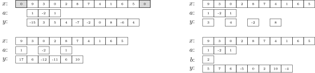
A worked example for a one-dimensional convolution operation is shown in Figure 34. Notice that the output signal is shorter than the input signal. Specifically, for input signal of length \(n\) and kernel of length \(p\), the output signal will have length \(n - p + 1\). We will address a strategy of how this can be avoided later in the lecture.

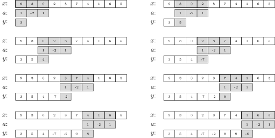
Instead of writing the convolution operation as an explicit summation, we can write it as a matrix-vector multiplication,

or in a more compact form,

Here the matrix \(A\), formed by rows containing shifted version of \(a^T\), is called a Toeplitz matrix. Viewing convolution in this way we see that convolution is a type of linear operator with weight sharing (i.e., sharing of parameters).

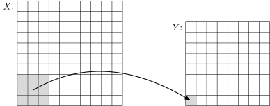
Convolutions on two-dimensional signals (or feature maps) follow much the same pattern as one-dimensional convolutions. Let \(X \in \reals^{n \times m}\) be an input signal and \(A \in \reals^{p \times q}\) be a filter. Then

for \(i = 1, \ldots, n - p + 1\) and \(j = 1, \ldots, m - q + 1\). Note that here the kernel is also two-dimensional and not only slides left-to-right over the signal, but also top-to-bottom, i.e., the kernel shifts over the plane. An illustration of two-dimensional convolution is shown in Figure 35. Once again, the output signal is smaller than the input signal.

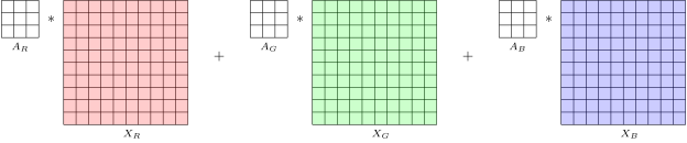
Now, recall from the first lecture that a feature map can have multiple channels. For example, an \(n\)-by-\(m\) colour image has three channels, \(X_R, X_G, X_B \in \reals^{n \times m}\), for red, green and blue colour information, respectively.

We can produce a feature map \(Y \in \reals^{(n-p+1) \times (m-q+1)}\) by convolving each channel with a filter \(A_R\), \(A_G\) and \(A_B\), and summing the output,

as depicted in Figure 36.

This is equivalent to stacking the channels into a 3-tensor and convolving with a 3D kernel. Convolutions on images and feature maps are defined as such. Let \(X \in \reals^{n \times m \times d}\) be an input signal and \(A \in \reals^{p \times q \times d}\) be a filter. Then

for \(i = 1, \ldots, n - p + 1\) and \(j = 1, \ldots, m - q + 1\). This is illustrated in Figure 37.

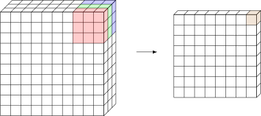
Observe that the input signal and kernel are both 3-dimensional tensors, but with same size third dimension (i.e., same number of channels \(d\)). This means that the filter kernel does not shift along the third dimension and the output signal only has one channel. Confusingly, this is called Conv2d in PyTorch.

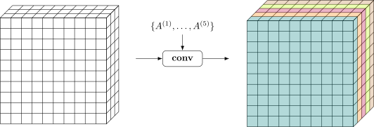
So far we have considered a single convolutional filter applied to the input signal or feature map. Convolutional layers in deep learning apply multiple filters and stack each of their single-channel outputs into a multi-channel tensor as illustrated in Figure 38. So, in general, we have as input a (\(C_{\text{in}} \times H \times W\))-tensor and apply \(K\) convolutional filter kernels, \(\{A^{(1)}, \ldots, A^{(K)}\}\), which are learned parameters of the layer. Here each \(A^{(k)}\) has shape \(C_{\text{in}} \times P \times Q\). Then, with appropriate padding (to be discussed shortly in Section 4.1.1), the layer will produce as output a (\(C_{\text{out}} \times H \times W\))-tensor with \(C_{\text{out}} = K\).

4.1.1 Padding, Stride, Dilation, and Bias

It is a little annoying that the convolution operation results in an output feature map that is smaller than the input feature map, i.e., reduces the signal size. This can be addressed by padding the input signal, typically done by appending zeros to the beginning and end of the signal, although other values are possible (such as cyclic padding or extending the end values). Given a filter kernel of length \(p\), appending \(p-1\) values will result in an output signal the same size as the input signal as shown in Figure 39.

Other variations of convolution are also possible. For example, we can change how far we move the convolutional filter for each successive output element. This is known as stride, and can be expressed mathematically for the one-dimensional case as,

for a stride of \(s\). This reduces the size of the output signal by roughly a factor of \(s\) and, similarly, reduces computation. Figure 39 shows an example for \(s = 2\).

Instead of skipping inputs as we move to the next output, we can also skip inputs when multiplying by filter coefficients. This is called dilation or (atrous) convolutions, and is equivalent to having a larger filter kernel with zeros inserted, but computationally more efficient. Mathematically, we have

for a dilation factor of \(d \geq 1\). Here \(d = 1\) indicates no dilation.

Last, it is standard to add a constant term, called a bias, to the result of the convolution, which can be written as,

for scalar parameter \(b\), which is learned during training along with the kernel parameters \(a\). The striking similarity to the affine transform, \(y = Ax + b\), within a multi-layer perceptron should not go unnoticed.

4.1.2 Back-propagation through Convolutions

To make convolutions learnable we need to be able to compute the derivative of the loss with respect to the kernel \(a\). Consider again the one-dimensional convolution,

and observe that each \(a_j\) affects every \(y_i\). As such, when back-propagating to compute the gradient of the loss with respect to \(a\) we need to sum the contributions for all the \(y_i\)’s. We have,

So it turns out that back-propagating through a convolutional layer in a deep learning network is itself a convolution operation!

Likewise, each \(x_k\) affects many \(y_i\). Here, however, the resulting expression has the convolution filter reversed

Similar expressions can be derived for higher-order convolutions.

4.1.3 Pooling

In addition to convolution layers, convolutional neural networks include pooling layers that reduce the size of features maps by aggregating feature values over a small local window, which is stepped across the feature map. This not only saves computation in downstream convolution layers but also acts to compress information and make the network more robust to data perturbations and small shifts within the scene. There are two common pooling operations. Average pooling computes the average of feature values in the window, where as max pooling takes the maximum value, and is hence a non-linear operation. These pooling methods are illustrated in Figure 40.

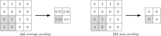
A \(2 \times 2\) window is very typical, with a stride of 2 (i.e., stepping the full window size), so that windows do not overlap. This results in downsizing a 2D feature map by a factor of four. Note that average pooling is the same as filtering (i.e., convolution) with a uniform kernel. For multi-channel feature maps, the pooling operation is applied separately on each channel.²

Since pooling layers do not have any learnable parameters we only need to be concerned with propagating gradients from the pooled outputs back to the inputs (so that parameters in earlier convolution layers can be learned). Calculating the gradients is fairly straightforward. Assuming that windows do not overlap (i.e., the stride is equal to, or greater than, the window dimensions), then for average pooling we have \(\fracdd[L]{x_i} = \frac{1}{N^2} \fracdd[L]{y_j}\) for window of size \(N \times N\) and where input \(x_i\) contributed to output \(y_j\). For max pooling the output gradient is copied to the argmax input and the other inputs get zero gradient, e.g., let \(y = \max\, \{x_i\}_{i=1}^{n}\). Then \(\fracdd[L]{x_i} = 0\) if \(y \neq x_i\) and \(\fracdd[L]{y}\) otherwise.³ If there are multiple inputs that tie for the maximum value then the gradient is split between them.

4.1.4 Convolutional Neural Networks

We now have all the ingredients necessary for constructing a convolutional neural network (CNN), which takes an image, i.e., \((3 \times H \times W)\)-tensor, and performs successive layers of convolutions, elementwise non-linear transforms (such as ReLU), and pooling. Early CNNs also performed features normalization, i.e., \(z \gets z / \|z\|_2\), but that is less common today. The final layers of a CNN take the last feature map, flatten it, and then process it through a multi-layer perceptron, also called fully-connected or dense layers in the context of CNNs. An architecture diagram for the famous AlexNet CNN [61] is shown in Figure 41. There are many other variants appearing in the literature and that we’ll see in future lectures.

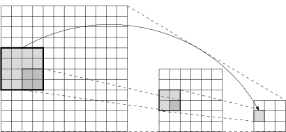
As can be seen in the diagram for AlexNex, the feature maps have smaller spatial dimension in later layers of the network compared to earlier layers. If we map back the size of the convolutional filter kernels to the original image then we see that a small kernel at a later layer in the network is processing data from quite a large area in the image. This is known as the receptive field of the filter. Figure 43 illustrates the idea using three successive layers of 2-by-2 pooling on a 12-by-12 image. By the third layer, each element of the feature map corresponds to data from a 4-by-4 region of the image, and so a 3-by-3 kernel applied on the third-layer feature map would corresponds to a receptive field of 12-by-12 in the original image. Thus, deeper models allow for consideration of larger receptive fields, which are necessary for capturing context, but without the computational demand of larger filters.

The first and still most common use of convolutional neural networks is for image classification—that is, given an image, predict the class that it belongs to (from some pre-defined set of categories). Instead of directly producing a class label, CNNs produce a probability distribution over classes, using a softmax function on the final layer logits, from which the most likely class can be trivially obtained. So for a \(K\)-class problem, the CNN backbone maps from a (\(3 \times H \times W\))-tensor representing the image to a \(K\)-vector as shown diagrammatically below:

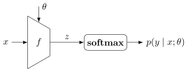
Here \(f\) represents the CNN model and \(\theta\) encapsulates all of the learnable parameters in the model, i.e., the convolution filter kernels and linear transforms in the final MLP layers. The size of the input to the CNN is fixed, and therefore images must be resized before processing. We will see later architectures that deal with inputs of varying sizes.

Common datasets used in image classification (see Figure 42) include MNIST [62], SVHN [76], CIFAR10/100 [60], ImageNet [21], Places365 [69], and many more. The first three are very small by modern standards and only used to try out new ideas, not in any real application. Training is done using stochastic gradient descent on the cross-entropy loss, and evaluation performed by reporting top-1 and top-5 accuracy on a held out test set. Here top-1 accuracy is the same as one minus the misclassification rate. Top-5 accuracy measures the number of times the true positive class appears within the set of five most probable classes (ranked by softmax probability, or equivalently, logit value). More nuanced metrics such as confusion matrices and precision-vs-recall will be discussed shortly.

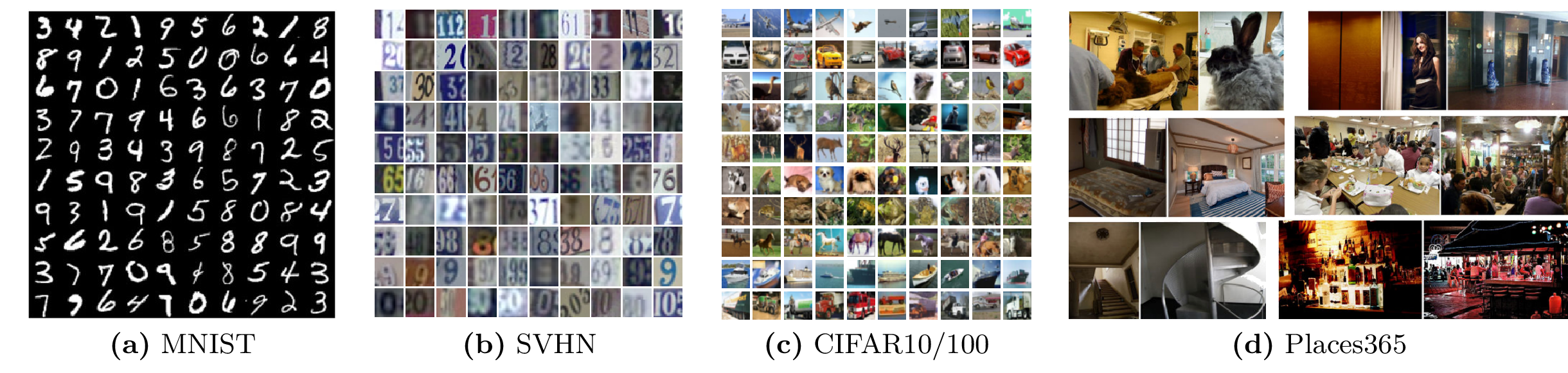
In addition to being a useful task in and of itself, image classification is often used as a test bed for developing new learning algorithms, and as a building block for more sophisticated image processing pipelines that we will see in later lectures.