Section 4.3
Other Architectural and Training Ingredients
4.3.1 Data Augmentation
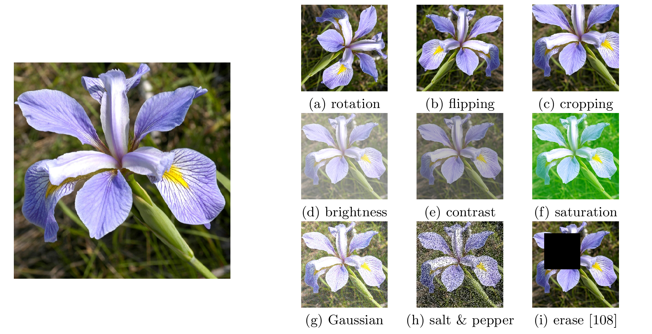
Data augmentation is a technique used to improve the robustness and generalization ability of neural networks by generating new training data from existing data. Since the model is now being asked—through training—to perform well on a larger set of data, overfitting is lessened. Transformations are applied to the existing training samples to create new samples with the same labels, i.e.,
where \(T\) is the data augmentation transformation function and \((x^{(i)}, y^{(i)})\) is a sample from the training batch. These transformations are typically applied on-the-fly as the data is loaded for a training iteration, and may be specific for a task, unlike general techniques such as regularization. They include a random element so that each time the transform is applied a slightly different data sample is generated. Example data augmentations for computer vision tasks are shown in Figure 46.
4.3.2 Batch Normalization
Recall from the last lecture that normalizing data helps convergence during training. Batch normalization (BN) [50] is a technique for on-the-fly centering and scaling of feature maps within the network. Consider a batch \(\cB = \{(x^{(i)}, y^{(i)})\}_{i=1}^{N}\) with intermediate features \(z^{(i)} \in \reals\), then BN calculates as its output
where
are the mean and standard deviation over the batch, respectively, and \(\gamma\) and \(\beta\) are learnable scale and offset parameters. For vector- or tensor-valued features, BN is applied to each index separately.
Running averages of \(\mu\) and \(\sigma\) are maintained for use during test time, since computing batch statistics at test time would violate the identically and independently distributed (i.i.d.) assumption of the test data.
4.3.3 Residual Connections and ResNet
One way to address the issue of diminishing gradients is via short-cut (or bypass or residual) connections that provide an identity transformation path in addition to some feature processing path. The ResNet block [41] shown in Figure 47 is a classic example. Let \(x\) be the input signal and let \(f\) be any neural network processing function, e.g., \(f(x) = C\sigma(Ax + b) + d\). Then, after adding a residual signal we have,
Note that in the original paper [41] ResNet was applied to the task of image classification. As such, the linear transformation was implemented as a 3D convolutional layer. The block also included batch normalization within the function \(f\).
If we now consider the gradient through the ResNet block we have,
As such, even if \(\ifracdd[f]{x}\) vanishes, we still have a gradient signal \(\ifracdd[L]{z}\) propagating through to the input. He et al. [41] showed that it is possible to train networks with a thousand layers using this trick by stacking successive ReNet blocks (see Figure 48). Today ResNet models are one of standard backbone architectures for all sorts of deep learning applications, going under the monikers of ResNet18, ResNet34, ResNet50 and ResNet101, which denote the number of layers.
![General form of a ResNet [41] block, which include a short-cut connection from the input. The linear layers can be either convolutional layers or fully-connecte](assets/diagrams/3544dce3fcf1ce61.svg)
It is quite easy to implement a ResNet block in PyTorch. Here we present code for a very basic convolutional version with batch normalization.
class BasicResNetBlock(nn.Module):
    """Example convolutional ResNet block."""

def __init__(self, in_planes, out_planes):
    super().__init__()

    self.conv1 = nn.Conv2d(in_planes, out_planes, kernel_size=3, stride=1, padding=1)
    self.bn1 = nn.BatchNorm2d(out_planes)
    self.relu = nn.ReLU(inplace=True)

    self.conv2 = nn.Conv2d(out_planes, out_planes, kernel_size=3, stride=1, padding=1)
    self.bn2 = nn.BatchNorm2d(out_planes)

def forward(self, x):

    f = self.bn2(self.conv2(self.relu(self.bn1(self.conv1(x)))))
    z = f + x
    y = self.relu(z)

    return y