Section 5.1
Region-CNN Family of Detectors
The first successful neural network object detector model was the R-CNN model proposed by Girshick et al. [30], although it was only partially end-to-end trainable. The basic idea is shown in Figure 56(a) and follows the recipe that we have been discussing thus far. Namely, the model is comprised of a CNN backbone that is pre-trained on the ImageNet dataset for image classification. Selective search [99] is used to propose rectangular regions and image crops are then resized to 227-by-227 pixels independent of the bounding box aspect ratio, and processed by the CNN backbone to obtain a 4096-dimensional feature vector per crop. Linear classification (called a support vector machine in the original paper) and bounding box regression branches operate on this feature representation of the image crop.
To obtain good results the bounding box branch predicts a transformation \((\Delta x, \Delta y, \Delta w, \Delta h)\) of the proposed region \(b = (x, y, w, h)\) as
where the translation \((\Delta x, \Delta y)\) is proportional to the box size \((w, h)\), and the scale transformation \((\Delta w, \Delta h)\) is in log-space. This makes the transformation invariant to re-scaling of the image.
![R-CNN, Fast R-CNN and Faster R-CNN networks for object detection. Images courtesy [29, 30, 85]](assets/diagrams/090509924c52bbe0.png)
One of the drawbacks of the R-CNN model is that the convolutional neural network backbone is repeatedly applied to every single proposed bounding box. This is computationally wasteful, especially for bounding boxes that are overlapping. A successor to R-CNN called Fast R-CNN [29] solves this problem by introducing region-of-interest (RoI) pooling (see Figure 56(b)). The idea is to first process the full image through the CNN backbone to obtain a 7-by-7 feature map. Bounding box proposals are projected onto the feature map and pooling performed per projected box proposal to obtain the region’s feature vector representation, which is then passed to the classification and bounding box regression branches as before.
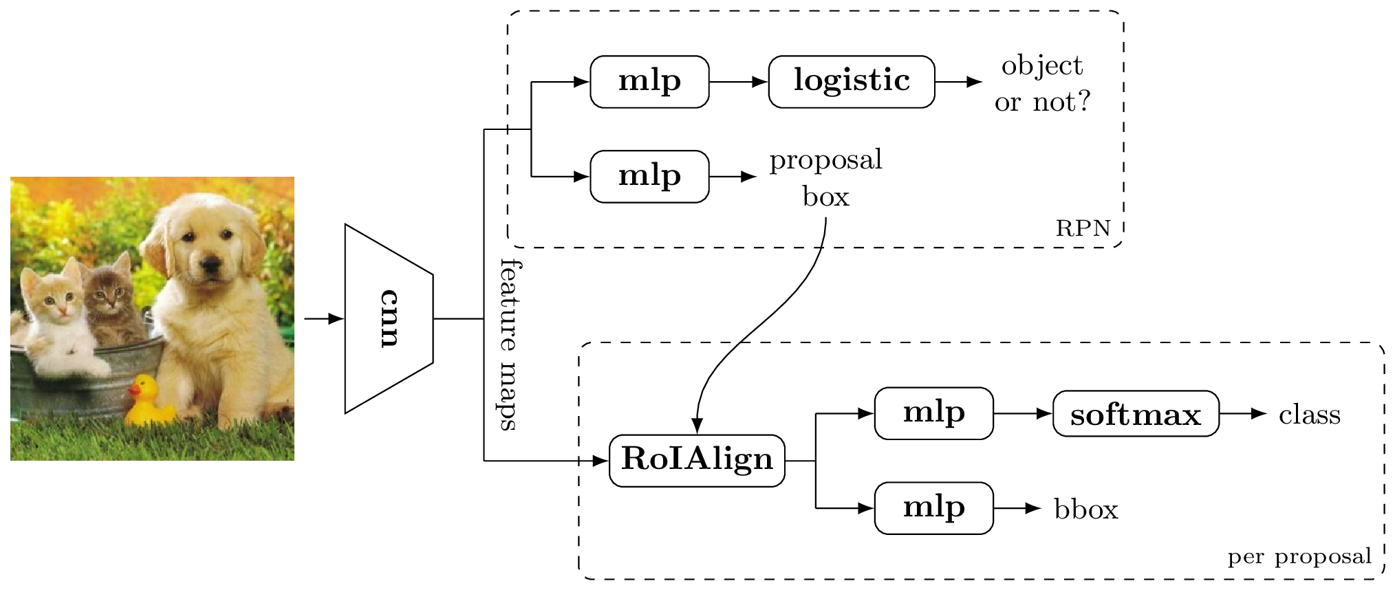
Just one problem remains: the model requires pre-processing of the image to obtain bounding box proposals, which as we will see is the main computational bottleneck. The Faster R-CNN model [85] shown in Figure 56 incorporates a region proposal network (RPN) that operates on the convolutional neural network feature map to do away with selective search pre-processing. This network predicts and scores bounding box proposals as it processes the image. Importantly, it uses the same CNN backbone allowing computation to be shared between region proposals and region classification.
5.1.1 RoIPool and RoIAlign Details
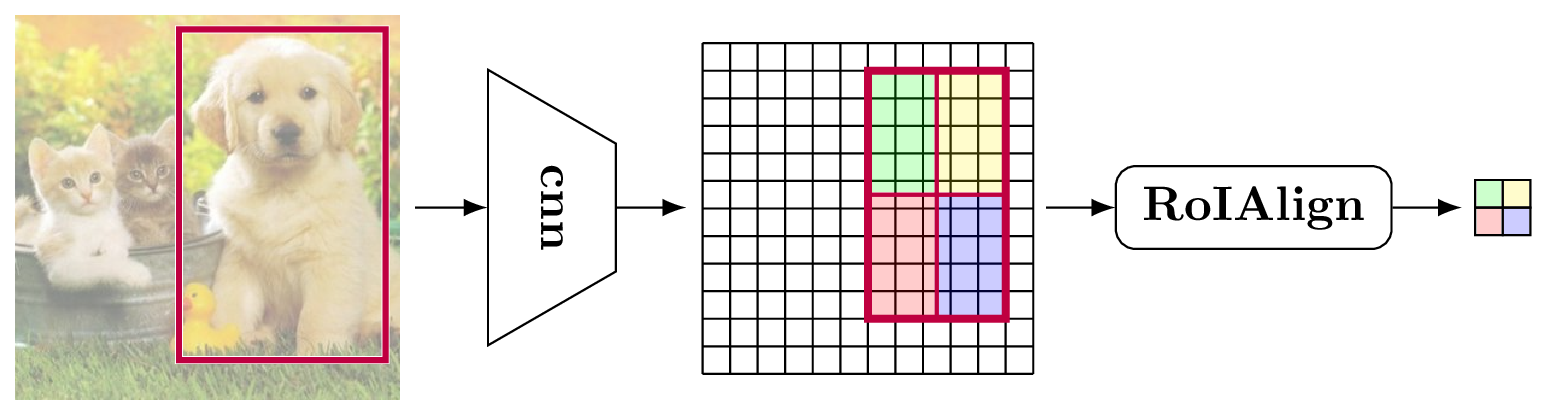
RoIPool and RoIAlign are operations that allow feature maps computed by the backbone CNN over the whole image to be pooled over an arbitrary rectangular region within it. The proposal regions in image coordinates are first projected onto the feature map. For RoIPool the projected region is snapped onto the feature map grid, whereas for RoIAlign the coordinates of the projected bounding box remain fractional and bilinear interpolation is used to align the feature map to the region. Max pooling is then applied over projected subregions (with all channels pooled independently). See Figure 57. This produces a fixed size output feature map that is independent of the size of the original proposed bounding box, and hence can be used by a downstream multi-layer perceptron for classification or bounding box regression. The feature map used in Fast R-CNN is 512-by-7-by-7.
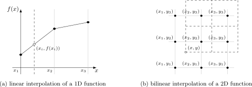
Bilinear interpolation is a general technique for estimating a function value between discretely sampled points. Let us start by considering the simpler problem of linearly interpolating between any two points on a one-dimensional function \(f: \reals \to \reals\) as shown in Figure 58(a). Picking a point \(x\) between two points \(x_1\) and \(x_2\) we have the interpolated value of the function at \(x\) as the convex combination of the function values \(f(x_1)\) and \(f(x_2)\),
where \(\alpha = \frac{x_2 - x}{x_2 - x_1}\) is the relative weight assigned to the first point (and \(1 - \alpha = \frac{x_1 - x}{x_2 - x_1}\) is the weight assigned to the second point). Note the inverse relationship between the weight and distance to the points.
We can extend this idea to the case of a two-dimensional function \(f: \reals^2 \to \reals\) defined on integer coordinates as illustrated in Figure 58(b). Bilinear interpolation allows us to compute function values at fractional coordinates by taking the weighted average of the four neighbouring points where nearer points are given proportionally higher weight. Here we first linearly interpolating along the \(x\)-direction to estimate the function at points \((x, y_1)\) and \((x, y_2)\), and then linearly interpolate between these two points to get the function value at \((x, y)\).1 The first interpolation gives,
where \(\alpha_1 = \frac{x - x_1}{x_2 - x_1}\) and \(\alpha_2 = \frac{x_2 - x}{x_2 - x_1}\). The second interpolation gives,
where \(\alpha_{ij} = \frac{|(x_i - x)(y_j - y)|}{(x_2 - x_1)(y_2 - y_1)}\) and \(f_{ij} = f(x_i, y_j)\). By studying this expression we can see that bilinear interpolation sums the function values at each corner point weighted by the relative area to the opposite point, e.g., \((x_2 - x)(y_2 - y) / (x_2 - x_1)(y_2 - y_1)\) is the weight used for \(f(x_1, y_1)\).
The expression above can be rewritten into a succinct matrix form,
for any point \((x, y) \in \reals^2\) lying within a box defined by integer coordinates \((x_1, y_1)\) and \((x_2, y_2)\) for the bottom-left and top-right corners, respectively.
5.1.2 Region Proposal Network Details
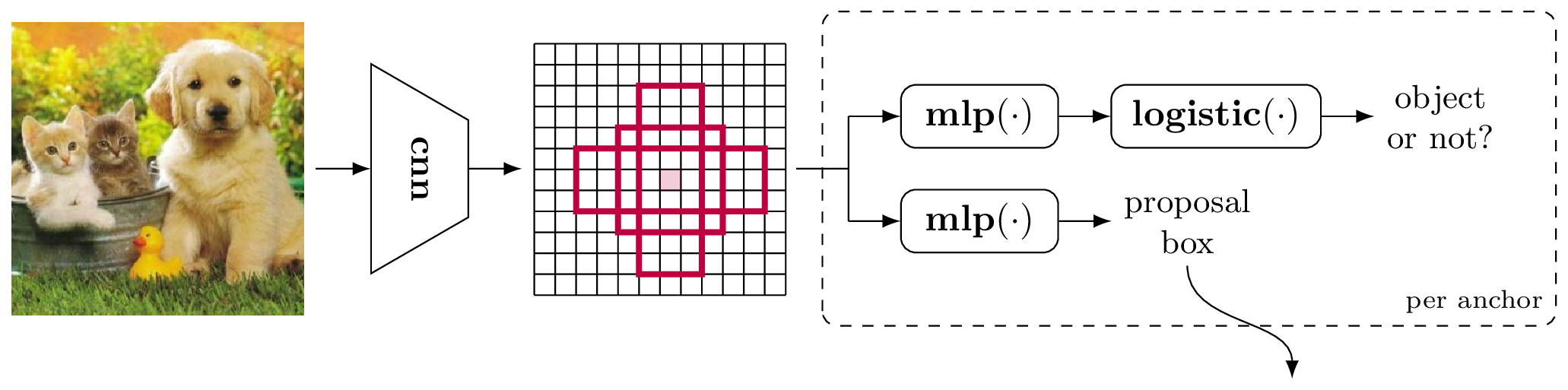
The region proposal network (RPN) in Faster R-CNN associates anchor boxes with each location in the feature map obtained from the backbone networks. These anchor boxes are of various sizes and aspect ratios, centered on the feature map location. See Figure 59. A multi-layer perceptron is used to classify each anchor box as either containing an object or not. For positive boxes, a second multi-layer perceptron regress bounding box transformation as described above for the R-CNN model.
The top-\(k\) scoring proposal boxes are fed to an RoIAlign module (along with feature map) to produce a feature representation for the corresponding bounding box. The model is trained end-to-end using a weighted combination of four loss components that include a binary cross-entropy loss and a transformation regression loss on anchor boxes, and multi-class cross-entropy and bounding box regression on proposals.
Putting all of these components together we arrive at the Faster R-CNN architecture shown in Figure 60. The CNN backbone processes the entire image to produce a feature map; the region proposal network generates bounding boxes; each proposed bounding box is fed to RoIAlign, which pools over the associated region in the feature map for classification and bounding box regression.
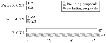
Including region proposals into the same deep learning model as the bounding box classifier (and regressor) makes a significant difference to inference speed. Shown in Figure 61 is the time taken by different models in the R-CNN family to process a single image. Pre-processing the image to obtain selective search bounding box proposals takes approximately two seconds per image. This is a bottleneck in the Fast R-CNN model, which is alleviated in the Faster R-CNN model. As we will see later, the accuracy of the model (Faster R-CNN) is also slightly improved, although this could be attributed to multiple factors.
- 1. Alternatively we could first interpolate in the \(y\)-direction at points \((x_1, y)\) and \((x_2, y)\) and then interpolate between these points to get the same result.