Section 5.6
Semantic Segmentation
Think back to the task of object detection from earlier in the lecture. The definition of the task requires that we place a bounding box around objects found in the scene. But this presents a problem for detailed analysis because it still leaves ambiguous which pixels within the bounding box belong to the object of interest as shown in Figure 69. Some pixels will belong to the background (or unknown objects), and in cases of overlapping bounding boxes, some pixels will belong to other objects. Semantic segmentation aims to solve this problem by assigning a category label (from a predefined set of known categories) to every pixel in the image. Note that semantic segmentation does not distinguish between different instances of the same object category so only partially addresses the issue of ambiguity caused by overlapping bounding boxes (i.e., when the categories are different).
Common datasets used for semantic segmentation research include MSRC [17], COCO [66], and Cityscapes [16], all of which have had their pixels painstakingly annotated by human labelers.

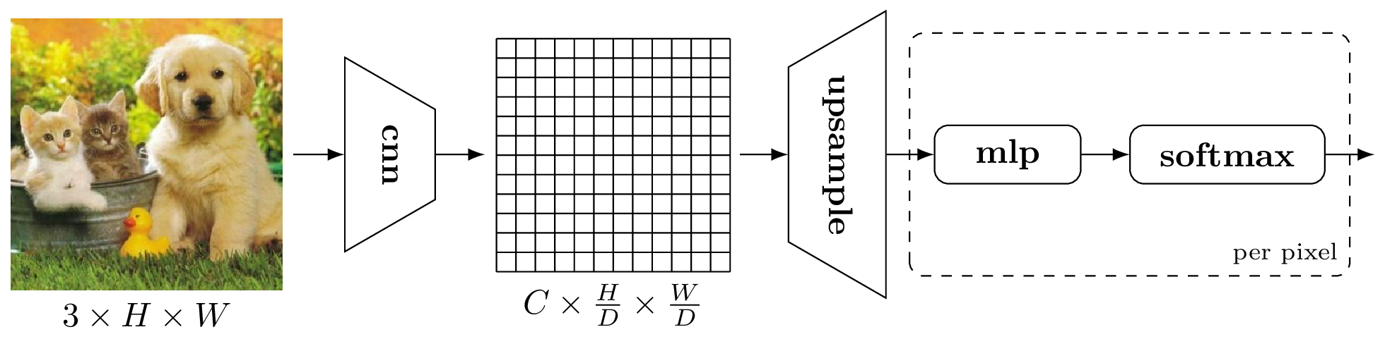
As we have seen convolutional neural networks are very good at processing images to produce features. However, the pooling layers reduce the feature map size so that we do not have a one-to-one correspondence between features and image pixels. For example, we may start with an \(H \times W\) colour image and end up with a \(C\)-channel \(\frac{H}{D} \times \frac{W}{D}\) feature map, where \(D > 1\) is the downsampling factor. This is a problem if we want to classify pixels individually. One solution, illustrated in Figure 70, is to upsample the feature maps back to the original resolution of the image. The resulting \(C\)-dimensional features at each feature map location can then be passed through a multi-layer perceptron (MLP) to obtain per-pixel classifications. Long et al. [68] showed that these per-pixel MLPs can be implemented efficiently using 1-by-1 convolutions allowing for arbitrary sized images to be processed.
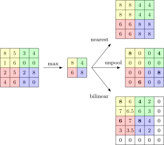
There are several options for upsampling the feature maps as shown in Figure 71. The simplest approach is nearest neighbour (also known as piecewise constant) upsampling. Here each element in the upsampled feature map takes its value from the closest location in the downsampled map. Treating the indices of elements in the downsampled map as integers and those in the upsampled map as fractional, we can write nearest neighbour upsampling as
where the operator \(\lfloor \cdot \rceil\) rounds its argument to the nearest integer. So, for example, the \((1.5, 1)\)-th element lies halfway between the \((1, 1)\)-th and \((2, 1)\)-th elements, and takes the value of the \((2, 1)\)-th element.1 If, in the case of max pooling, we happened to remember the index of the maximum element when downsampling then we can simply restore the value to that location when performing upsampling, and setting the remaining elements to zero. This is known as unpooling and requires some housework in storing the maximizing indices in addition to the feature maps throughout the convolutional neural network layers. Yet another option is to perform bilinear interpolation,
over a 2-by-2 grid as discussed in the previous lecture, or bicubic interpolation, which is popular in photo editing tools when resizing images, but requires a 4-by-4 grid.
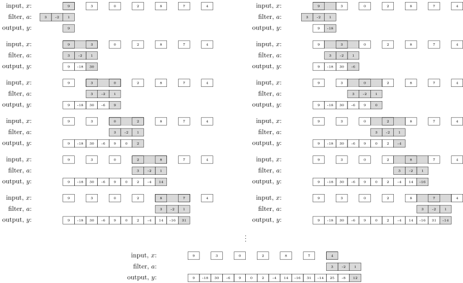
A more flexible approach is to learn the upsampling function. In deep learning this is done via transposed convolutions, sometimes called deconvolution. Note that this is not the same as a mathematical inverse. Let \(x \in \reals^n\) be an input signal, \(a \in \reals^p\) be a filter kernel, and \(s \geq 1\) be a stride. Mathematically, we can write the transposed convolution operator as
where \(x_{\frac{i-j+s}{s}}\) is defined to be zero if the index is fractional or greater than \(n\).
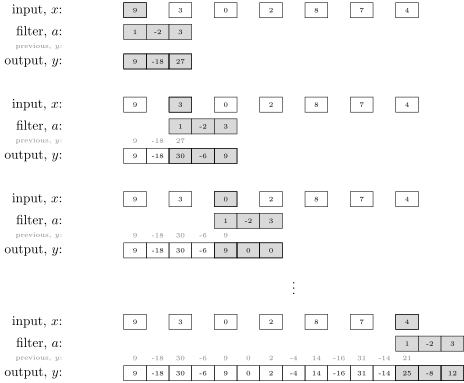
The operation is perhaps easier to understand through a worked example. There are two ways the computation for transposed convolution defined above can be implemented. Figure 72 shows a worked example for filter \(a = (1, -2, 3)\) with stride of 2 using the reverse strided convolution method. Figure 73 shows the same operation but implemented using the scale, shift and sum (or accumulate) method. Both methods produce the same result—as must be the case. Observe also that the output signal is larger than the input signal.
Just like standard convolutions, we can view transposed convolution as a linear operator. Recall that for a one-dimensional convolution (with stride = 1) we have as a matrix equation,
We can similarly write the one-dimensional transposed convolution (with stride = 1) as,
In compact form we have, \(y^{\text{conv}} = Ax\) and \(y^{\text{trans}} = A^T x\), and hence the name transposed convolution.
Long et al. [68] proposed three variants of the fully convolutional network (FCN) architecture as shown in Figure 74. All variants apply learned upsampling (i.e., transposed convolutions) to different pooling layers for pixelwise prediction. The first variant, FCN-32s, applies upsampling to the fifth pooling layer, requiring 32 times upsampling. The second variant, FCN-16s, applies two times upsampling to the seventh convolutional layer, which is also then added to the forth pooling layer. The resulting sum is then upsampled 16 times to get back to the original image size. The last variant, FCN-8s, adds the (upsampled) seventh convolution layer and forth pooling layer to the third pooling layer, which is then upsampled eight time to reach the original image size. In summary, the FCN architecture predicts pixel labels on upsampled feature maps from different pooling layers. These predictions are then fused via pixelwise summation as a way of averaging coarse and fine level predictions.
![The fully convolutional network (FCN) architecture of Long et al. [68]](assets/figures/fcn.png)
A similar yet more flexible approach combines feature maps of the same size from the downsampling branch with the upsampling branch, and only makes predictions on the combined feature maps of the final layer. Consider a sequence of downsampled and upsampled feature maps
with \(\textbf{shape}(F_{\ell}^{\text{E}}) = \textbf{shape}(F_{\ell}^{\text{D}})\). The so-called skip connections compute \(F_{\ell-1}^{\text{D}}\) using \(F_{\ell}^{\text{D}} \oplus F_{\ell}^{\text{E}}\) instead of just \(F_{\ell}^{\text{D}}\), where \(\oplus\) denotes concatenation along the feature dimension. This propagates contextual information from the “encoder” to the “decoder” layers of the network as illustrated schematically in Figure 75.
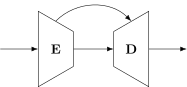
The very popular U-Net [87] architecture, shown in Figure 76, uses this idea but does not require the feature maps to be the same size. Indeed, the feature maps on the encoder side are larger and than on the decoder side and the skip connection crops the larger feature map before concatenating with the smaller one. The network was originally proposed for medical image analysis but is now the backbone in many pixel-to-pixel computer vision tasks including semantic segmentation, image denoising, and image generation.
![The U-Net architecture proposed by Ronneberger et al. [87] uses skip connections to propagate information from the encoder to the decoder layers](assets/figures/unet.png)
- 1. Here we have chosen to round 0.5 up to the nearest integer.