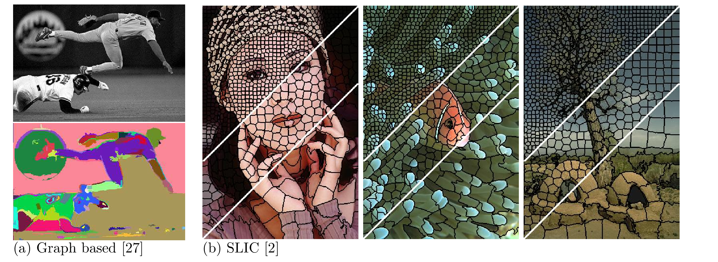
Unsupervised over-segmentation is a method for breaking an image up into small regions of uniform colour or texture, also known as superpixels. There have been many different algorithms proposed in the literature and we will only present two here, neither of which are data driven and, hence, do not involve any learning (hence are unsupervised).
Figure 65: Superpixel algorithms break an image up into many small coherent regions.
Felzenszwalb and Huttenlocher [27] proposed an efficient graph-based image segmentation algorithm that is the method used by Selective Search [99] for bounding box proposals in R-CNN discussed in the last lecture. In their method, the image is treated as graph \(G = \langle V, E \rangle\), where pixels (and incrementally built segments) are nodes in the graph, \(v_i \in V\), connected to their neighbouring pixels (or segments). The edges in the graph, \(E\), are weighted by similarity \(w_{ij}\) (where we set \(w_{ij} = \infty\) if \(v_i\) and \(v_j\) are not adjacent). The graph is then partitioned into segments based on within- and between-segment similarity as shown in Figure 66.
Figure 66: Toy example of graph-based segmentation [27]. Nodes are annotated with their index (i.e., identifier). Edges are annotated with their weights, \(w_{ij}\). The graph is partitioned into segments satisfying the boundary condition, \(\textbf{diff}(C_a, C_b) > \min\left\{\textbf{int}(C_a) + k/|C_a|,\, \textbf{int}(C_b) + k/|C_b|\right\}\) for \(k=10\).
Let \(C \subseteq V\) be a segment (or component) in the graph. We define two measures,
where \(|C|\) denotes the number of nodes in \(C\), and \(\textbf{mst}(C)\) is a minimum spanning tree of \(C\). Note that \(\textbf{int}(C)\) is infinite if \(C\) is disconnected.
We want to find a partitioning of the graph into segments such that the following boundary condition is satisfied between any two distinct components \(C_a\) and \(C_b\) in the segmentation,
where \(\tau(C) \triangleq k / |C|\) prevents degenerate solutions (e.g., singleton segments). An example partition that satisfies this condition is shown for a toy graph in Figure 66.
It turns out that a partitioning can be found that satisfies the boundary condition using a greedy algorithm that iteratively merges clusters of pixels, starting from each pixel being placed in its own cluster. The following pseudo-code outlines the algorithm, which can be implemented very efficiently using a disjoint set data structure, \(O(|V| \log |V|)\).
1:functionGraphBasedSegment(graph, \(G = \langle V, E \rangle\), and threshold, \(k\))
2:/* initialize */
3:for all nodes \(i \in V\) do
4:set pixel to its own segment, \(C_i = \{i\}\) with \(\textbf{int}(C_i) = 0\)
5:end for
6:for all edges \((i,j) \in E\) do
7:set edge weights \(w_{ij}\) to be square distance between pixels \(i\) and \(j\) in colour space
8:end for
9:sort edges \((i, j)\) by weight in non-decreasing order
10:/* merge clusters */
11:for all edges \((i,j)\) do
12:let \(C_i \ni v_i\) and \(C_j \ni v_j\)
13:if \(C_i \neq C_j\) and \(w_{ij} \leq \min\left\{\textbf{int}(C_i) + \frac{k}{|C_i|},\, \textbf{int}(C_j) + \frac{k}{|C_j|} \right\}\) then
14:merge \(C_i\) and \(C_j\)
15:set \(\textbf{int}(C_i \cup C_j) = w_{ij}\)
16:end if
17:end for
18:return segmentation \(S = (C_1, C_2, \ldots)\)
19:end function
A worked example showing each step of the algorithm for the previous toy example is shown in Figure 67.
Figure 67: Worked example graph-based segmentation algorithm of Felzenszwalb and Huttenlocher [27] for a 5-by-3 image with 4-connected neighbourhood and \(k=10\). The algorithm proceeds from left-to-right then top-to-bottom choosing the lowest cost edge to merge segments. Where there are multiple edges all with the same lowest cost, one is chosen arbitrarily. Edges are annotated with similarity score. Segment membership is indicated by colour and the minimum spanning tree indicated using bold edges.
The graph-based algorithm of Felzenszwalb and Huttenlocher [27] produces irregularly shaped regions as can be seen in the example in Figure 65. An alternative algorithm that produces more regular shaped superpixels, and is also very efficient, is the simple linear iterative clustering (SLIC) algorithm of Achanta et al. [2]. In their approach \(k\)-means clustering is repeatedly applied, limited to a local neighbourhood in a \(2S \times 2S\) patch around each centroid, with \(S = \sqrt{WH/K}\) where \(K\) is the number of desired superpixels. Clustering is done using a distance metric defined on 5-dimensional colour and spatial features, \((l, a, b, x, y)\) as
where \(m\) controls the compactness of the superpixels, trading off spatial versus colour distances. The algorithm is summarized by the pseudo-code below and illustrated in Figure 68.
1:functionSLIC(grid size, \(S\))
2:/* initialize */
3:set cluster centroids \(C_k\) by sampling pixels on a regular \(S \times S\) grid▷ (avoids putting centroid on
4:move centroids to lowest image gradient in \(3 \times 3\) neighbourhood▷ an edge or noisy pixel)
5:/* iterate */
6:repeat
7:assign best matching pixel from \(2S \times 2S\) neighbourhood for each cluster \(k\)
8:recompute centroid \(C_k\) for each cluster
9:until no change (or maximum iterations reached)
10:/* finalise */
11:tidy up orphaned and small clusters
12:return superpixels \((C_1, C_2, \ldots)\)
13:end function
Figure 68: Illustration of local neighbourhood clustering within the SLIC [2] algorithm. Any pixel within the dashed region can be assigned to cluster \(C_6\), allowing pixels to move from the eight neighbouring clusters \(C_1\), \(C_2\), etc.
![Toy example of graph-based segmentation [27]. Nodes are annotated with their index (i.e., identifier). Edges are annotated with their weights, . The graph is pa](assets/diagrams/40a78f5b96f3b9c8.svg)
![Worked example graph-based segmentation algorithm of Felzenszwalb and Huttenlocher [27] for a 5-by-3 image with 4-connected neighbourhood and . The algorithm pr](assets/diagrams/c243cda3c5f6979d.svg)
![Illustration of local neighbourhood clustering within the SLIC [2] algorithm. Any pixel within the dashed region can be assigned to cluster , allowing pixels to](assets/diagrams/f651d45b0a32ac63.png)