Section 6.1
Recurrent Neural Networks
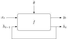
A recurrent neural network (RNN) is a model that processes an input sequence one element at a time. It also takes part of the output and feeds it back into itself as an additional input. This allows it to keep state information based on previously processed inputs. A schematic diagram of an RNN is shown in Figure 81. Let \(x_t\) be the \(t\)-th element in the input sequence and \(h_{t-1}\) be the partial output from the previous time-step. Then the output of the RNN is computed as,
where the same function \(f\) with same parameters \(\theta\) is applied at each time-step. Variable \(h_t\) is called the hidden or latent state. It is initialized to some nominal value, \(h_0\), at the start of the sequence. Note that as defined, the RNN produces one output for every input, and is therefore a many-to-many model. It can be made into a many-to-one model by waiting until the entire sequence is processed and discarding all but the last output.
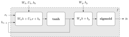
A concrete example of an early recurrent neural network proposed by cognitive scientist Elman [25] is shown in Figure 82. Here the latent state and output are computed as,
respectively. This is just a variant of the multi-layer perceptron where the hidden state \(h_t\) and output \(y_t\) are elementwise non-linear transformations of linear functions of the current input \(x_t\) and previous hidden state \(h_{t-1}\). The learnable parameters are \(W_h\), \(U_h\), \(b_h\), \(W_y\) and \(b_y\).
We can view convolution over an arbitrarily long input signal as a very simple recurrent neural network. For brevity let us consider the one-dimensional case. Let \(a \in \reals^p\) be a \(p\)-length filter kernel, and let \(x_t \in \reals\) be the value of the input signal at time \(t\). Initialize \(h_0 = (0, \ldots, 0) \in \reals^{p}\). Then we can implement convolution as a recurrent network with
where the output is delayed by \(p-1\) time steps, which is how long it takes for the model to process the receptive field of the filter kernel. However, general RNNs are much more expressive.