Section 6.5
Language Models
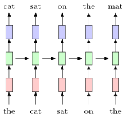
Language models are sequence-to-sequence models that produce an output for each input in the sequence. Specifically, a language model predicts the next token in a sequence where a token can be an individual character, an complete word, or anything in between (e.g., an \(n\)-gram) that is suitably encoded as a vector (to be discussed shortly). At each time step, an RNN outputs a probability distribution over all possible tokens. For example,
where each element in \(y_t\) represents the probability that the next token has index corresponding to that element and is constructed as a single-layer perceptron (logistic regressor) with the RNN hidden state as input. We then take the most likely token as the predicted output or sample a token weighted by its probability. A depiction of a language model is shown in Figure 87. Since the RNN is producing a probability distribution, it can be learned using a cross-entropy loss. Note that the target output at time \(t\) is the same as the model’s input at time \(t+1\). As such, language models can be trained in a self-supervised manner on a large corpus of text.
6.5.1 Encoding Words as Vectors
Neural networks process numerical data; they cannot process symbolic data such as words. As such we need a mechanism to encode (and decode) words as vectors. Consider a vocabulary \(\cV\) consisting of \(m\) words. We can encode each word in \(\cV\) using one-hot encoding as illustrated below,
That is, the \(i\)-th word in the list maps to \(e_i = (0, \ldots, 1, 0, \ldots) \in \reals^m\).
Since the first layer of an RNN is typically a linear layer, \(z = Ax + b\), with \(A \in \reals^{n \times m}\), we can map directly from the word to the output of this linear layer.1 The \(i\)-th word mapping becomes
where \(a_i\) is the \(i\)-th column of \(A\). Note that \(b\) can be absorbed into \(A\) as \(A \gets A + b \ones^T\) for the special case of multiplying only by one-hot vectors, and so can be ignored for the purpose of learning embeddings. So, in summary, instead of going through the step of encoding words using a one-hot vector, we can just directly learn word embeddings, where \(z_i \in \reals^n\) represents the \(i\)-th word in the vocabulary. The matrix \(A\) is sometimes called the embedding matrix.
6.5.2 Training Language Models
Getting back to language model training, we mentioned above that they can be trained using a cross-entropy loss. Roughly speaking, we wish to learn the parameters of the model that best predict the next token in a sequence, a task known as next-token prediction. The approach follows a teacher-forcing paradigm, where irrelevant of the next-token distribution predicted by the model at any time step, the learning algorithm provides the (supervised) ground-truth token as input for the next time step. The objective is then to minimize the cross-entropy loss over next-token distributions for all time steps,
where \(w_t\) is the index of the correct ground-truth word (or token). The loss function is defined over all parameters \(\theta\), which include \(A\), \(b\), and the parameters of recurrent function \(f\).
As we’ve already discussed, back propagating through long temporal sequences can be problematic from a vanishing gradient perspective, and also from a memory perspective—we have to store all intermediate calculations from the forward pass. One way to get around this difficulty when training language models is to chunk long sequences into segments of length \(T\), by caching \(h_s\) for some \(s > 0\) and treating it as a constant for the next chunk,
The word embeddings are usually pre-trained via a separate process and kept frozen during language model training. We will discuss learning embeddings later in this lecture and in the next lecture.
6.5.3 Auto-regressive Generation and Beam Search
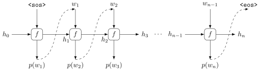
Output sequences can be generated from recurrent neural networks in an auto-regressive fashion as shown in Figure 88. We have already seen that the recurrent network for a language model predicts a probability distribution over the next word in the sequence given the current state and previous word, \(p(w_t \mid h_t, w_{t-1})\). To generate an output sequence we initialize the latent state \(h_0\) and set the previous word to a special start-of-sequence token (<sos>). We then sample the first word from \(p(w_1 \mid h_0, \texttt{<sos>})\). This word (and the updated latent state) is then provided as input for the second time step. Proceeding in this way we keep sampling the next word \(w_t\) from \(p(w_t \mid h_t, w_{t-1})\). Generation stops when the model samples another special token, the end-of-sequence token (<eos>).
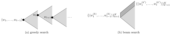
One problem with auto-regressive generation is that it is greedy. Even if we sample the most likely word at each time step, \(w_t \in \argmax_w p(w \mid h_t, w_{t-1})\), this may not result in the highest likelihood overall sequence, \(\langle w_1, w_2, \ldots, w_n \rangle\). This may happen, for example, if a word early in the sequence has high probability given the preceding text, but then results in a fairly uniform distribution over future words for the remainder of the sentence.
Beam search is a technique used to mitigate this problem. Here a set of \(K\) partially generated sequences, called a beam, is maintained, i.e., \(\{\langle w_1^{(k)}, \ldots, w_{t-1}^{(k)} \rangle\}_{k=1}^{K}\) at time step \(t-1\). Then at time step \(t\) we sample several next words for each partial sequence in the beam. The newly created \(t\)-length sequences are scored and all but the top \(K\) discarded. In principle, we are reducing the set of \(mK\) newly created sequences (\(m\) next words from a vocabulary of size \(m\) for each of the \(K\) partial sequences in the beam) back down to a set of \(K\) (high scoring) sequences in the beam. An illustration of this process and comparison with greedy search is shown in Figure 89.
A typical scoring metric for partial and full sequences \(\langle w_1, w_2, \ldots, w_t \rangle\) is the joint log-probability,
Other more sophisticated scoring functions that take into account sequence length can also be used. At the end of the generation process, the most likely sequence from the set of \(K\) completed sequences is chosen as the model output.
An interesting extension to beam search proposed for guided caption generation is constrained beam search [4]. The idea here is that we want to constrain the output sequence to contain a certain word, or more generally match a pattern encoded by some regular expression. However, since the sequence is generate auto-regressively, we cannot expect the pattern to necessarily be present at the start of the sequences. Indeed, forcing the pattern to appear at the start may result in a very low probability sequence instead of allowing the pattern may appear anywhere. To get around this difficultly Anderson et al. [4] propose to maintain multiple beams, each beam representing partially matched patterns.2 As words are added to the sequences in the beams, the longer sequences can move to different beams indicating that a pattern is now satisfied or not. Once generation of the sequences completes, only sequences in beams representing matched patterns are candidates for the model output. A subtle tweak to the method just described is to additionally force sampling of transitions between beams (i.e., states in the regular expression automaton) at each time step, thus ensuring that sequences satisfying the constraint always exist.