Section 6.2
Back-propagation Through Time
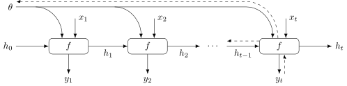
To train a recurrent neural network we need to back-propagate through each time step. We do this by unrolling the network to a given time horizon,
and then back-propagating through the unrolled sequence of operations. Note that output \(y_t\) depends on parameters \(\theta\) and latent state \(h_{t-1}\), which in turn depends on \(\theta\) and \(h_{t-2}\), which in turn depends on \(\theta\) and \(h_{t-3}\), and so on. In other words, the parameters affect the output through direct and multiple indirect paths. Assuming that the loss is only applied to the last output, \(y_t\), we have
where we have recursively invoked the calculation of direct and indirect gradients. If the loss function were applied to intermediate outputs then these would also need to be accounted for in the gradient calculation. An illustration of the unrolled network and the concept of back-propagation through time is shown in Figure 83.
One of the issues with unrolling a recurrent model is that it creates a very deep network if we unroll for a long time horizon. As we have seen in previous lectures, this exacerbates the vanishing and exploding gradient problem. Consider the gradient contribution from a timestep \(s < t - 1\) for the concrete example RNN shown in Figure 82,
Each term in the product \(\frac{\partial h_{\tau+1}}{\partial h_\tau}\) is obtained by differentiating the tanh activation function,
Using the result, \(\frac{\textrm{d}}{\textrm{d}z} \tanh(z) = 1 - \tanh^2(z)\), we have
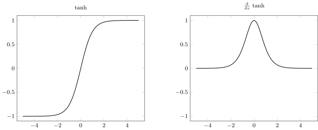
where \(h^2_{\tau + 1}\) is the vector \(h_{\tau+1}\) with its elements squared. Figure 84 plots both the tanh function and its derivative. We can observe from the plots that if any \(h_{\tau + 1}\) is close to \(\pm 1\) or \(\sigma_{\text{max}}(W_h) < 1\), then the gradient will vanish. Furthermore, if all \(h_{\tau + 1}\) are close to zero and \(\sigma_{\text{max}}(W_h) > 1\), then the gradient will explode. Here \(\sigma_{\text{max}}\) is the maximum singular value of \(W_h\) (and has no relation to the same symbol \(\sigma\) used to denote the logistic function in earlier lectures and elsewhere in this lecture).