Section 11.1
Background and Revision
Before embarking on deep learning models for learning distributions from data (or more precisely how to sample from such distributions), we first revise some important background material.
11.1.1 Gaussian Distributions
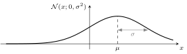
Gaussian distributions are ubiquitous in statistics, science and engineering. You should easily recognize the classic bell shape of the one-dimensional Gaussian shown in Figure 132.
A multivariate Gaussian distribution with mean \(\mu \in \reals^n\) and covariance \(\Sigma \in \reals^{n \times n}\) has form
which we often write as \(\cN(x; \mu, \Sigma)\) or \(\cN(\mu, \Sigma)\) for short. Here \(|\Sigma|\) denotes the determinant of the covariance matrix and together with the other terms in the scaling factor in front of the expression (called the partition function), acts to normalize the distribution so that it integrates to one.
The Gaussian distribution has some useful properties:
- Elements of \(x\) are independent, i.e., \(p(x_i, x_j) = p(x_i) p(x_j)\), if and only if the covariance matrix is diagonal
- The conditional distribution \(p(x \mid y)\) of jointly Gaussian random variables \((x, y)\) is Gaussian
- The marginal distribution \(p(x) = \int p(x, y) \, \textrm{d}y\) of jointly Gaussian random variables \((x, y)\) is Gaussian
A special case is the zero mean, unit covariance Gaussian, \(\cN(0, I)\). We can sample from an arbitrary Gaussian by transforming a sample from the unit Gaussian. That is, we can sample \(x \sim \cN(\mu, \Sigma)\) as
where \(\epsilon \sim \cN(0, I)\). This is sometimes called the reparameterization trick, which we will use it often in this lecture.
11.1.2 Jensen’s Inequality
Jensen’s inequality is a result from convex analysis that states that for any convex function \(f(x)\) and any distribution \(p(x)\) we have
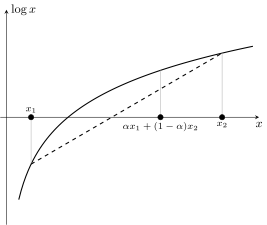
For concave functions the inequality is reversed. Specifically \(\log x\) is a concave function of \(x\), so
A good way to remember the direction of the inequality is through the visualization in Figure 133. Here the function is concave and the line between any two points, representing the expected value of the function \(E \left[ \log x \right]\), lies below the function itself \(\log E \left[ x \right]\).
11.1.3 Variational Lower Bound

Let \(X\) and \(Z\) be two random variables modeled by some joint distribution \(p_{\theta}\). A graphical model [58] illustrating the factored distribution \(p_\theta(Z) p_\theta(X \mid Z)\) is shown Figure 134. Suppose we only get to observe \(X\). We want \(p_\theta(X)\) to be a good probabilistic model of our observed data, \(\cD\). We can try doing this by choosing \(\theta\) that maximizes the probability of the observed data as per the maximum likelihood principle,
Unfortunately this is difficult to compute in general as it requires integrating out \(Z\),
Later we will see how to get around this difficulty by introducing a lower bound on \(\log p_\theta(x)\).