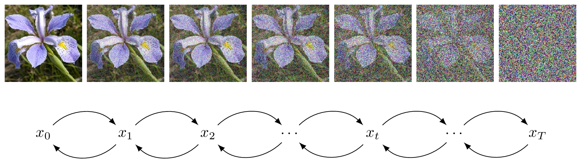
Figure 136: The forward diffusion process (top) generates noise from data, \(\text{data}, x_0 \in \reals^n \to \text{noise}, x_T \in \reals^n\). The reverse diffusion process (bottom) recovers a sample from the data distribution from noise, \(\text{noise}, x_T \in \reals^n \to \text{data}, x_0 \in \reals^n\).
Diffusion models are generative models that learn to reverse a gradual noise corruption process. Starting from real data \(x_0\), a forward diffusion process progressively adds Gaussian noise over many timesteps until the data becomes nearly pure noise. A denoising diffusion probabilistic model (DDPM) then learns the reverse process: given a noisy sample \(x_t\), a neural network predicts either the original signal or the added noise so that the model can iteratively denoise samples back into realistic data. This is shown in Figure 136 and an example denoising network architecture in Figure 137.
Figure 137: Neural network architecture for producing a sample \(x_{t-1}\) from \(q(x_{t-1} \mid x_t, t) = \cN(f_\mu(x_t, t; \theta), f_\Sigma(x_t, t; \theta))\). The reparameterization trick is used so that we can back-propagate through \(\mu\) and \(\Sigma\). The model is often simplified to assume spherical covariance, \(\Sigma = \sigma_t^2 I\) with predetermined fixed \(\sigma_t\).
Training is typically performed by minimizing a simple mean-squared error objective on the predicted noise, while generation begins with Gaussian noise and repeatedly applies learned denoising steps. DDPMs are highly stable to train and can generate extremely high-quality samples, although sampling is often computationally expensive because it requires many sequential denoising iterations. Training and sampling algorithms are provided below.