Section 11.3
Variational Auto-Encoders
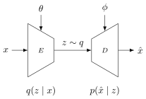
A standard auto-encoder learns a compressed representation of data by mapping an input \(x\) to a latent representation \(z\), and then reconstructing the input as \(\hat{x}\). The architecture consists of and encoder \(E\) and decoder \(D\) with parameters \(\theta\) and \(\phi\), respectively. The encoder computes,
and the decoder reconstructs the input as
The model is trained to minimize reconstruction error, e.g.,
over a dataset of examples \(\cD\).
Although auto-encoders can learn compact latent representations, the latent space is often poorly structured. Small perturbations in \(z\) may produce unrealistic outputs, making standard auto-encoders unsuitable for generative modeling.
A variational auto-encoder (VAE) addresses this issue by making the latent representation probabilistic. Instead of mapping an input to a single point \(z\), the encoder predicts a probability distribution, \(q(z \mid x)\), and the decoder then models \(p(x \mid z)\) as shown in Figure 135. Thus, the encoder produces a distribution over latent variables and the decoder generates data conditioned on sampled latent variables.
Typically, the encoder outputs the parameters of a Gaussian distribution,
where \(\mu(x)\) is the latent mean and \(\Sigma(x)\) is the latent covariance matrix, both estimated by the encoder and provided as output. In practice \(\Sigma(x)\) is assumed to be diagonal for efficiency.
A discussed in the preliminaries, a latent sample can be obtained using the reparameterization trick,
where \(\epsilon \sim \cN(0, I)\). This sampled latent vector is then passed through the decoder to generate \(\hat{x}\).
The model is trained by deriving a variational lower bound known as the evidence lower bound (ELBO). Briefly, we introduce an approximate posterior distribution \(q(z \mid x)\) to the true posterior \(p(z \mid x)\) and rewrite the marginal likelihood as
where we have used Jensen’s inequality on Line 3 to obtain a tractable bound. The second term is a Kullback-Leibler divergence \(D_{\text{KL}} \left(q(z \mid x; \theta) \,\|\, p(z) \right)\). This allows us to write the VAE training objective as
where the first term is a reconstruction loss that encourages the decoder to accurately reconstruct the input \(x\) from the latent representation \(z\). For Gaussian decoders this reduces to a squared-error loss. The second term provides regularization so that there is meaningful interpolation between latent points, stable sampling, and generative capability. Without the regularization term the latent space can become fragmented and difficult to sample from. A full training algorithm is shown below.
Although VAEs are stable and principled generative models, they have several weaknesses. First, the reconstructions are often blurrier than the outputs from other generative models such as GANs or diffusion models because they optimize a likelihood-based objective. Second, they are susceptible to posterior collapse where the decoder ignores the latent variables entirely, \(q(z \mid x) \approx p(z)\). This is especially common when the decoder is too powerful.
Despite these limitations VAEs have found application in a number of areas, and extended to allow the incorporation of a conditioning signal (resulting in CVAEs) and quantized latent spaces (VQ-VAEs), which give sharper reconstructions and mitigate against posterior collapse. VQ-VAEs are widely used in audio generative systems and sequences requiring tokenized latent representations [100].